2. Virtual Water Trade

The concept of virtual water was formally named in 1993 by British geographer, John Anthony Allan. This came about while researching how water scarce countries in the Middle East were still able to meet the food needs of their people despite not having enough water to grow their own food. These countries instead import food from water rich countries. In this way, the embedded water in the food is transferred from one country to another. The transfer of this hidden water through the import and export of goods (foods and all other goods) is called virtual water trade (VWT).

Virtual water trade puts the concept of virtual water into practical use. It allows countries to assess how much water they would use by growing crops themselves based on their own growing conditions compared to the water they gain (virtually at least) if they imported the same number of crops from a different country.

The amount of virtual water embedded in a crop varies through time and location. The preceding chapters have explained how climatic conditions change rates of evapotranspiration (ET), and how different farming practices, soil health, and irrigation efficiencies can alter how much water will be needed to grow a given crop. This knowledge can be applied to how the virtual water content of a crop will change if grown in one location versus another.

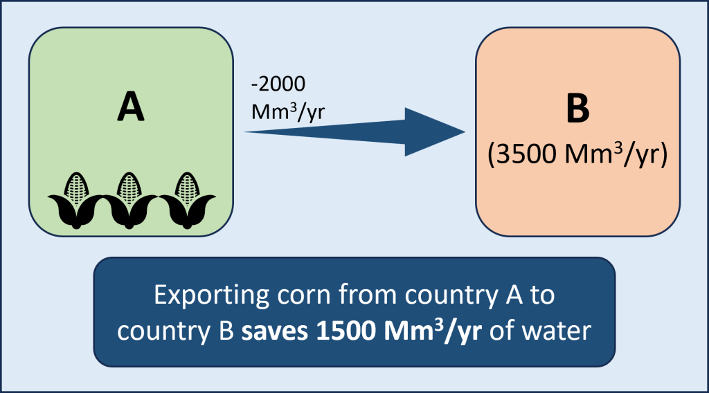
The example in Figure 2D.2.1 below illustrates this by using corn production in two hypothetical countries, A and B. Country A has climatic conditions that lead to lower ET rates and has broadly healthier soil and more efficient irrigation practices than country B. This means in country A less water is needed per acre of corn and therefore the virtual water (VW) content of corn from country A is lower. Country B is water stressed and chooses to import corn from country A. The amount of corn it imports has a VW content of 2000 Mm3/y (million cubic meters per year). This is how much water country A had to use to produce this corn. If that same volume of corn was grown in country B, it would have required 3500 Mm3/y. Importing corn instead of growing it in country B has created a net savings of virtual water of 1500 Mm3/y (3500 Mm3/y – 2000 Mm3/y = 1500 Mm3/y).

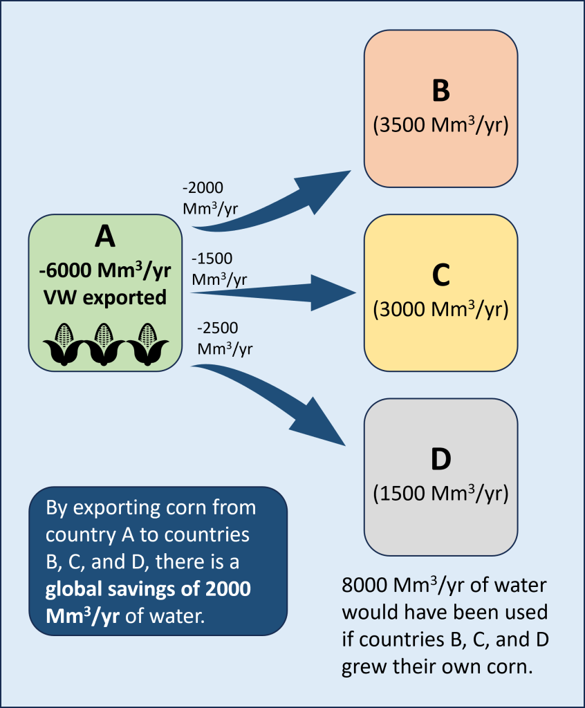
This VWT analysis can be expanded further to look at whether imports and exports between multiple countries result in global water savings or losses. If the total amount of VW in products exported from one country into multiple others is overall less than the combined water those countries would have used to produce their own goods, then this is an overall savings of virtual water. Figure 2D.2.2 demonstrates this by expanding on the corn example above and including exports of corn from country A to not only country B but countries C and D as well. With this expanded look at VWT, country A embeds a total of 6000 Mm3/y of virtual water in corn that it exports, but if the other three countries were to have grown that corn themselves it would have required 8000 Mm3/y. So, this VWT results in a global saving of 2000 Mm3/y of virtual water.

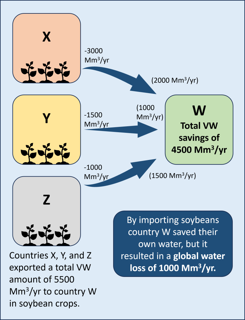
Virtual water trade does not always lead to net savings of water. A country that is water scarce may choose to limit what they grow and instead import crops to save water. However, if the country they are importing those crops from is also water scarce or has poor growing conditions then this virtual water trade may result in a net loss of water globally. This is illustrated in Figure 2D.2.3 where country W is importing soybeans from countries X, Y, and Z. If country W had grown its own soybeans, it would have used 4500 Mm3/y of water. By importing it has saved this water for other activities. However, while there is a gain of virtual water for country W, in looking at where the soybeans were imported from and how much water those countries used to grow the soybeans, an overall global loss of water can be seen. Countries X, Y, and Z exported a combined total of 5500 Mm3/y of virtual water resulting in a net loss of 1000 Mm3/y of virtual water (4500 Mm3/y – 5500 Mm3/y = -1000 Mm3/y).

The map below shows the global virtual water trade of agricultural and industrial products from 1996-2005 (Figure 2D.2.4). Countries shaded in green are net exporters of virtual water (negative import values on the scale bar), while countries in shades of orange and red are net importers of virtual water. The main net virtual water exporters were the United States, India, China, Canada, Brazil, Argentina, and Australia, whereas main net virtual water importers were Japan, United Kingdom, much of western Europe, Algeria, and Saudi Arabia. The black arrows demonstrate some of the major water flow directions. While countries like the United States and China have both imports and exports of virtual water owing to having large economies, they still both export more than they import.

Analyzing virtual water trade can lead to minimizing water usage globally, if this knowledge is applied to discourage the production of high virtual water products in water scarce regions and instead encourages production in water rich regions or regions where the growing conditions are most ideal. This would create a more sustainable global use of water and reduce water stress and ecosystem damage in water scarce regions.

This seems easy on paper, but hard to implement in real life as it is a complex issue. The sociopolitics involved in trade means no country, even one that is highly water stressed, wants to rely only on imports to feed its population. Food independence, not water availability, is a major driver of large-scale agriculture. In addition, reliance on imports has other ramifications. It means farmers within the importing countries would lose their livelihoods, likely forcing them to move into urban areas which then increases water pressure in cities. If the importing country is relying on finances from a particular industry (let’s say oil exports) to fund the purchase of food imports and the oil reserves dry up, then they will no longer have the means to purchase food. In the exporting countries, oftentimes crops for export are subsidized, which encourages farmers to grow them. This alters the water use and food production within the exporting country and can lead to overuse of water resources and groundwater depletion.

There are many pros and cons associated with the virtual water trade and finding ways to use water sustainably while also diminishing any negative consequences of trade will only get more challenging as climate change continues to alter water resources on the planet.

References

Hoekstra, A. Y., & Mekonnen, M. (2012). The water footprint of humanity. Proceedings of the National Academy of Sciences of the United States of America, 109(9), 3232–3237. https://doi.org/10.1073/pnas.1109936109