3. Modern and Projected Consequences of Climate Change
The planet is already experiencing some of the disastrous consequences of climate change from increased temperatures to drought to wildfires. Climate models project how those consequences will continue or change into the future. Throughout the following discussion on modern and projected consequences of climate change, the five scenarios (SSP1-1.9, SSP1-2.6, SSP2-4.5, SSP3-7.0, and SSP5-8.5) will be referenced where applicable to demonstrate the range of consequences that could be possible based on human behavior and mitigation efforts in the future. Below are some, but definitely not all, of the consequences the planet faces as a result of climate change.
3.1 CO2 Emissions and Atmospheric Concentrations
Atmospheric carbon dioxide concentrations are rising because of human activity. This is a direct result of increased carbon dioxide emissions largely from the burning of fossil fuels. CO2 emissions began increasing following the start of the Industrial Revolution around 1750 and as a result, atmospheric concentrations also began to rise. At first, emissions rose slowly to about 5 billion tons per year in the mid-1900s before rising to more than 35 billion tons per year by the early 2000s (Figure 3D.3.1, grey line). The rate of rising emissions is unprecedented in Earth’s history. The closest analog to the current rise in CO2 emissions was during the PETM, however, the current rise in emissions is almost 10 times more than during the PETM. The rising emissions have resulted in an accelerating rate of rise in atmospheric CO2 concentrations (Figure 3D.3.1, blue line), with current atmospheric concentration of CO2 above 420 parts per million.
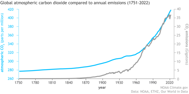
Present day carbon dioxide concentrations are higher than at any point in human history and are higher than any point since about 3 million years ago, before the start of the Pleistocene Glaciation, when global surface temperature was about 2.5 – 4 degrees Celsius (4.5 – 7.2 degrees Fahrenheit) warmer than the pre-industrial era.
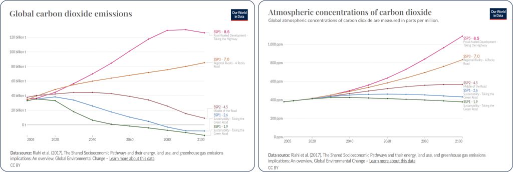
The actions humans take as populations rise and energy demand increases could push human emissions of CO2 over 120 billion tons per year by 2100 and lead to atmospheric concentrations of over 1,000 ppm (Figure 3D.3.2, pink lines). This is a CO2 concentration that has not happened since the PETM when temperatures were over 34 degrees Celsius (over 60 degrees Fahrenheit) warmer.
This is the worst case scenario brought on by a fossil fuel driven society, but even in a sustainable (SSP1-1.9 and SSP1-2.6) future where emissions are curbed quickly, there will still be a rise in atmospheric CO2 through at least 2050 before concentrations level off and start to fall. Only with the most aggressive mitigations (SSP1-1.9) will atmospheric concentrations fall below present-day levels by 2100. In a middle of the road world (SSP2-4.5), where emissions drop slowly starting in 2050, atmospheric concentrations will continue to rise, slowly leveling off in the year 2100 (Figure 3D.3.2). The time lag between cutting emissions and when concentrations start to level or fall is due to the long atmospheric lifetime of CO2.
3.2 Temperature
Global average temperatures have been steadily increasing as atmospheric CO2 rises. The Paris Agreement set climate goals to limit average temperature rise to well below 2°C above pre-industrial levels with strong efforts to limit temperature rise to 1.5°C. With increased research on the consequences of climate change, the goal of limiting temperature rise to 1.5°C has become a strong focus in recent years.
Of the 5 scenarios discussed in the 6th IPCC report, only one of them, SSP1-1.9, keeps temperature rise to below the 1.5°C threshold. SSP2-2.6 keeps temperature rise below 2°C, but the remaining 3 scenarios all project temperature rises above this of 2.63°C for SSP2-4.5, over 4°C for SSP3-7.0, and over 5°C for SSP5-8.5 (Figure 3D.3.3).
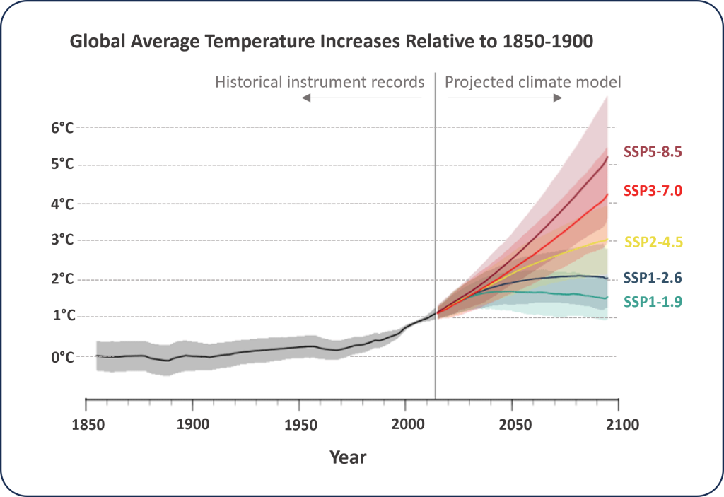
The planet has already warmed, on average, more than 1°C above the pre-industrial era, and 2023 marked the first year on record where every single day in the year exceeded 1°C above pre-industrial levels. Almost 50% of the days were more than 1.5°C warmer than pre-industrial and for the first time ever, two days were more than 2°C warmer – these occurred in November.
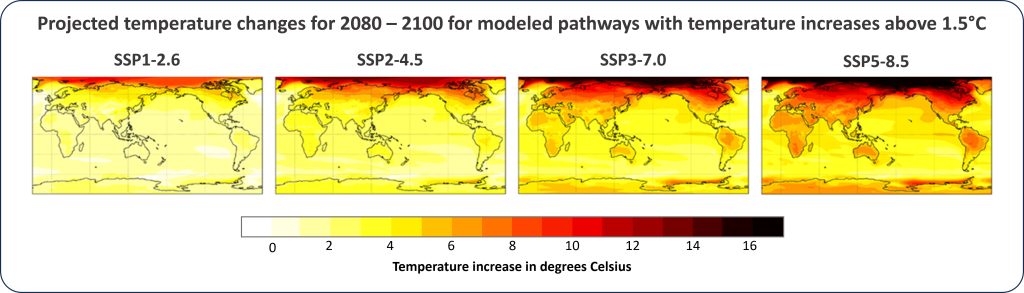
As with all consequences of climate change, rising temperatures are not even across the planet and some areas will experience more rapid temperature increases than others. Generally, temperatures are projected to rise more quickly over land than over the oceans and arctic regions will experience the largest temperature increase. Figure 3D.3.4 illustrates the spatial variation in temperature increases for the four scenarios that have average temperature increases above 1.5°C by 2100 (SSP1-2.6, SSP2-4.5, SSP3-7.0, and SSP5-8.5).
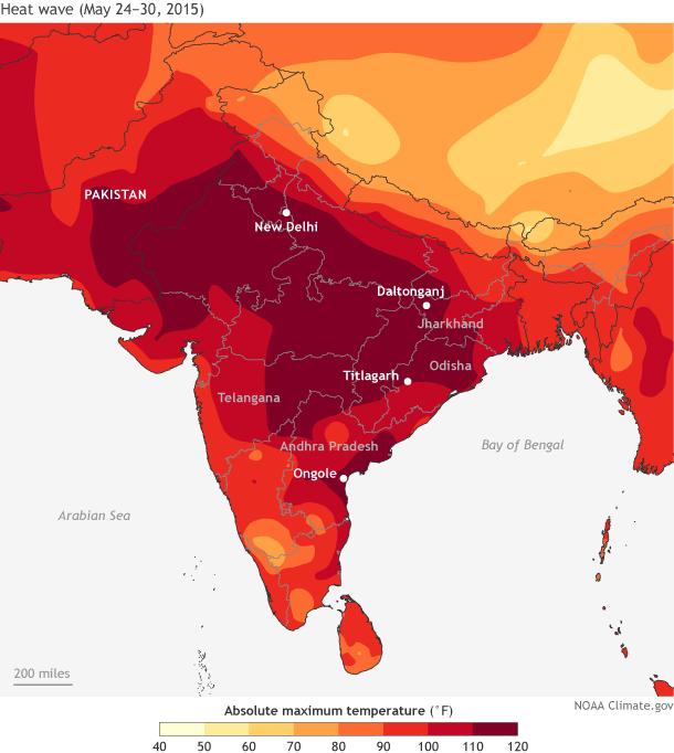
The times and locations of extreme temperatures, hottest days at mid latitudes and coldest nights at high latitudes, will be particularly effected. The mid latitude hottest days will have temperature increases up to 3°C (5.4°F) hotter at 1.5 degrees Celsius of warming and 4°C (7.2°F) warmer at 2 degrees Celsius of warming. These temperature increases will expose more people to severe heatwaves. With 2°C of warming, extreme heat waves, like the ones that have affected Pakistan and India in recent years may occur annually.
In May 2015 temperatures across parts of India and Pakistan reached over 45°C (113°F) (Figure 3D.3.5). Average temperatures across the region in May are typically 32°C-40°C (89-104°F). This lead to the deaths of over 2,500 people in India and about 2,000 people in Pakistan. In the Indian capital city, New Delhi, temperatures were hot enough that asphalt roads were reportedly starting to melt. The effects of high temperatures were compounded by humid conditions. In some areas, electricity failures related to the extreme temperatures also meant necessary cooling, such as home air-conditioning units, were not available, increasing the heat related deaths.
In March and April of 2022 another extreme heat wave hit, accompanied by temperatures higher than any in recorded history for these months in the area. Thankfully the associated death toll was lower, at 90, but extreme heat waves are expected to become the new normal if global temperatures continue to rise.
To keep temperatures from rising more than 1.5°C, global greenhouse gas emissions must be cut by 43% by 2030.
3.3 Freshwater
Water Availability and Droughts
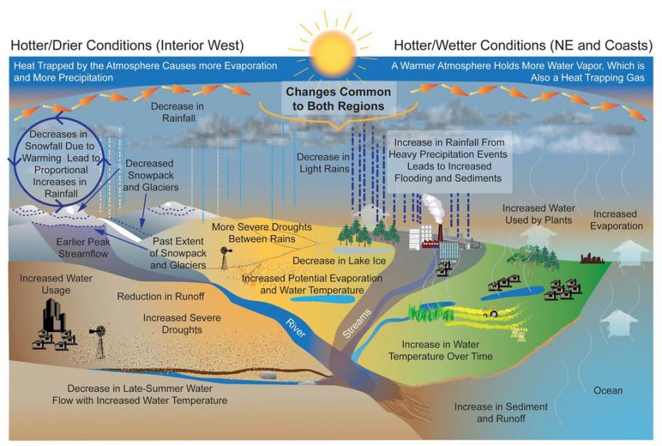
Higher temperatures brought on by climate change are expected to increase the stress on freshwater resources. The demand for water will go up while simultaneously shrinking the existing water supply. In some areas, higher temperatures drive increased evaporation leading to increased water stress and drought conditions. In the United States this is already happening across the west as seen in the Colorado River Basin. The high evaporation rates lead to increased atmospheric moisture and precipitation, so some areas will experience higher than normal precipitation. Increased temperatures also mean less precipitation is falling as snow and more is falling as rain, reducing the winter snowpack and spring runoff, which are important water sources for some river systems. Across the United States, hotter and drier conditions are projected across the interior of the country while hotter and wetter conditions are projected for the northeast and coastal regions (Figure 3D.3.6).
Changes in the trends of precipitation are already being seen and are projected to get worse as temperatures rise. Even in areas that overall are seeing unchanged volumes of precipitation, when and how that precipitation arrives has changed. Instead of small, steady amounts of rain or snow, storms are becoming larger, heavier downpours that punctuate dry, drought-like conditions. Large, heavy downpours cannot easily be absorbed by soil and instead lead to increased surface runoff and flooding conditions. So even areas where precipitation might increase because of climate change, soil moisture and drought can still be issues. In addition, increased surface runoff and flooding can stress water infrastructure and create or exacerbate water contamination issues.
Increased evaporation and decreased soil absorption cause decreased groundwater infiltration, so groundwater resources are also affected by changing precipitation patterns. Decreases in surface and groundwater resources will have lasting effects on agriculture, food supply, and human health.
If warming can be kept to 1.5°C, it is estimated that up to 270 million fewer people will be affected by water scarcity issues by 2050 compared to if climate warms by 2°C.
Storms
Higher air and sea surface temperatures increase atmospheric moisture. High sea surface temperatures also fuel the development of ocean storms such as hurricanes and cyclones. Therefore, as climate continues to warm, these storms are projected to have increased rainfall rates associated with them causing more flood damage once they make landfall. While the overall frequency of storms is not expected to significantly change, warmer sea temperatures are projected to fuel larger, more intense storms creating a larger proportion of category 4 and 5 storms. The latitudinal range over which these storms develop is also projected to increase as ocean temperatures increase.
Snow, Ice, and Permafrost
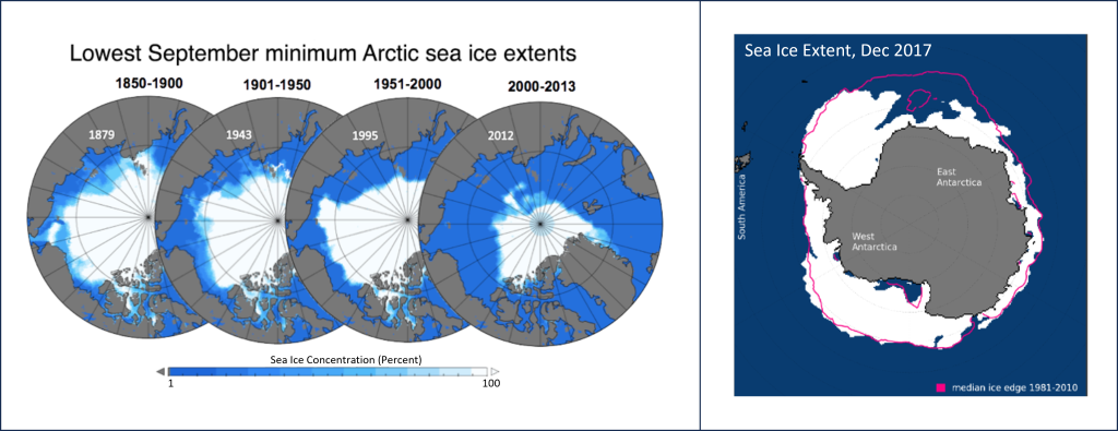
As climate warms, the snow season will continue to shorten, with snow accumulation beginning later and melting starting earlier. Snowpack is expected to decrease in many regions. Already the planet is experiencing reduced springtime snow cover, retreat of mountain glaciers, reductions in the Greenland and Antarctic ice sheets, and loss of Arctic sea ice. Figure 3D.3.7 illustrates the reduction in Antarctic sea ice during December and the reduction in Arctic sea ice during September, when northern hemisphere ice is at its minimum extent. Studies suggest the earliest occurrence of a totally ice-free September in the Arctic could occur in the 2020-2030s under all SSP scenarios, and that September would frequently be ice-free by mid-century with different durations and frequency depending on the scenario. At 1.5°C of warming the Arctic is expected to be ice-free once every century, but at 2°C of warming this will increase to being ice-free once every decade.
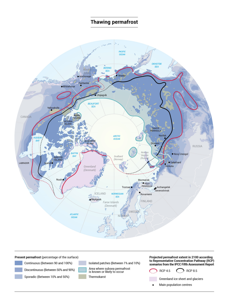
Permafrost is ground that is perpetually frozen, and it covers almost a quarter of the surface of all land mass in the northern hemisphere and contains close to 50% of all organic soil carbon (Figure 3D.3.8). If the permafrost stays frozen this carbon remains locked away but, as temperatures warm, the carbon can be released to the atmosphere in the form of methane and CO2. It is projected there will be widespread loss of near-surface permafrost by 2100 which not only releases greenhouse gases to the atmosphere but also impacts ecosystems and people living in the area.
As permafrost thaws, the ground becomes soft impacting infrastructure like buildings and roadways built on this ground. Cities and towns throughout the Arctic have been affected by this with damage to buildings causing a loss of housing and damage to road and railways cutting off important supply routes to remote areas. The thawing ground also becomes soft and swampy increasing the risk of flooding through these communities. Indigenous communities residing in the Arctic are particularly affected by having ancestral lands washed away or needing to relocate due to flooding. In addition, cultural lifestyles and practices that relied on the cold climate and frozen ground are being threatened. Practices such as storing food in the frozen ground are not possible if the permafrost melts, which means food stocks are at risk of rotting, leading to food insecurity.
Ice sheet dynamics are an active area of scientific study to determine where “tipping points” of ice loss will occur. Tipping points in the climate system are thresholds that once reached mean irreversible changes in the Earth system. Certain levels of ice sheet melting and permafrost thawing have already gone beyond their tipping points in the Earth system and even if climate cooled to levels below those which lead to the melting and thawing, this ice and permafrost would not reform. Curbing greenhouse gas emissions can help keep the planet from reaching new tipping points.
3.4 Oceans
Sea Level Rise
Rising sea level is because of a combination of thermal expansion of water and melting snow and ice. The
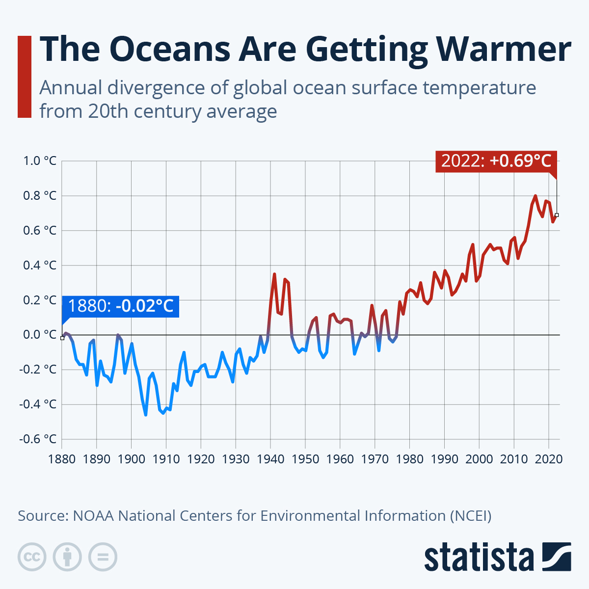
high heat capacity of water allows the oceans to store most, over 90%, of the excess heat added into the Earth system while having a much smaller change in temperature than would be seen if the atmosphere was storing this heat. The high heat capacity of water means that the same amount of energy used to raise ocean temperatures by 0.01°C (0.018°F) would increase atmospheric temperature by approximately 10°C. Ocean temperatures have risen by 0.8°C (almost 1.5°F) over the past century (Figure 3D.3.9). As water heats up it becomes less dense, therefore the same mass of water takes up more volume – this is thermal expansion and is estimated to be responsible for about 42% of sea level rise. The remaining 58% of sea level rise is due to new water being added into ocean basins from melting snow and ice, namely melting alpine glaciers and the two continental ice sheets on Greenland and Antarctica.

Sea level has risen over 250mm (over 9.8 inches) since 1880 (Figure 3D.3.10). Through this time, the rate of sea level rise has been increasing with an average rate of sea level rise of between 1 and 2 mm/year from 1901-2006 but this has drastically increased over the last ten to fifteen years and between 2013 and 2022 the rate of sea level rise rose to 4.62 mm/year.
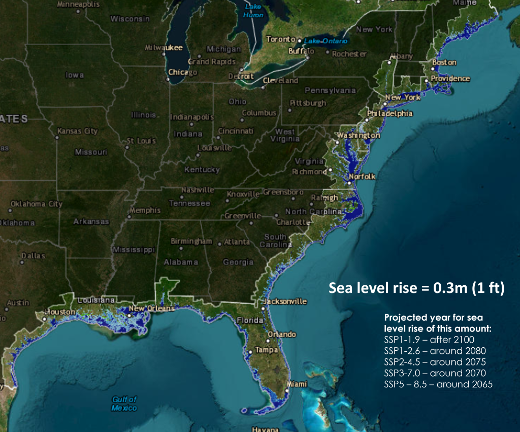
As temperatures continue to rise the contribution to sea level rise from the melting of ice sheets is projected to increase. The Antarctic and Greenland ice sheets store most of the land ice and have a sea level equivalent of over 65m (213ft). It is projected that if current emission levels remain, the planet will reach a tipping point by 2075 where complete melting of these ice sheets will become inevitable even if temperatures can ultimately be kept to only 1.5°C of warming by 2100. The complete melting of these ice sheets would take 10,000 years or more, but by 2100 sea level would rise by 0.3 to over 1.3m (1ft to over 4ft) depending on the emissions scenario modeled. Figure 3D.3.11 shows the land areas along the Eastern and Gulf Coast United States that will be inundated with water at 03.m (1ft) of sea level rise. While 1 foot of rise may not sound like much, for the low elevation areas this brings much higher risk of flooding from the inundation of sea water as well as more intense flooding brought onshore with tropical storms. This includes major cities along the East Coast, like Boston and New York all the way down to Miami and areas along the Gulf Coast. The generally steeper landscape of the West Coast of the United States means sea level rise will not flood the landscape as readily as the other coastlines.
Ocean Acidification
Ocean acidification is a reduction in the pH of the ocean over time. This is caused primarily by the uptake of CO2 from the atmosphere. Oceans absorb about 30% of atmospheric carbon dioxide, so as emissions and atmospheric concentrations grow, oceans absorb larger and larger amounts of CO2. Over the past 200 years, the average pH of the ocean has decreased from 8.2 to between 8.0 and 8.1 – this may not seem like a lot, but pH is measured on a logarithmic scale, so this equates to greater than a 30% increase in acidity.
pH scale reminder:
The pH scale runs from 0-14 with 7 being neutral. A pH value less than 7 is acidic and a value greater than 7 is basic. pH is the negative logarithmic measure of free hydrogen ions (H+), so more hydrogen ions means something has a lower pH value. Acids are compounds that will dissociate in a solution to release hydrogen ions while bases will bond with hydrogen ions to take them out of solution.
CO2 dissolves in ocean water (CO2(aq)) and reacts to create carbonic acid (H2CO3) which rapidly dissociates into bicarbonate (HCO3–) and a hydrogen ion. This can further dissociate to make carbonate (CO32-) and another hydrogen ion (Figure 3D.3.12). Carbonate ions are very important building blocks in the marine ecosystem as they combine with dissolved calcium in the water to create calcium carbonate – the mineral that composes coral reefs, shell material, and some plankton bodies. Bicarbonate does not dissociate completely, and most of the carbon in the ocean is in the form of bicarbonate. The ocean can buffer its pH, so that as pH increases (fewer H+, more basic), bicarbonate can dissociate and release hydrogen ions to lower the pH but as pH decreases (more H+, more acidic) carbonate ions will bond with H+ to create more bicarbonate and raise the pH. In this way the series of chemical reactions shown in Figure 3D.3.12 can run towards the right or the left as needed to keep the ocean at an appropriate pH.
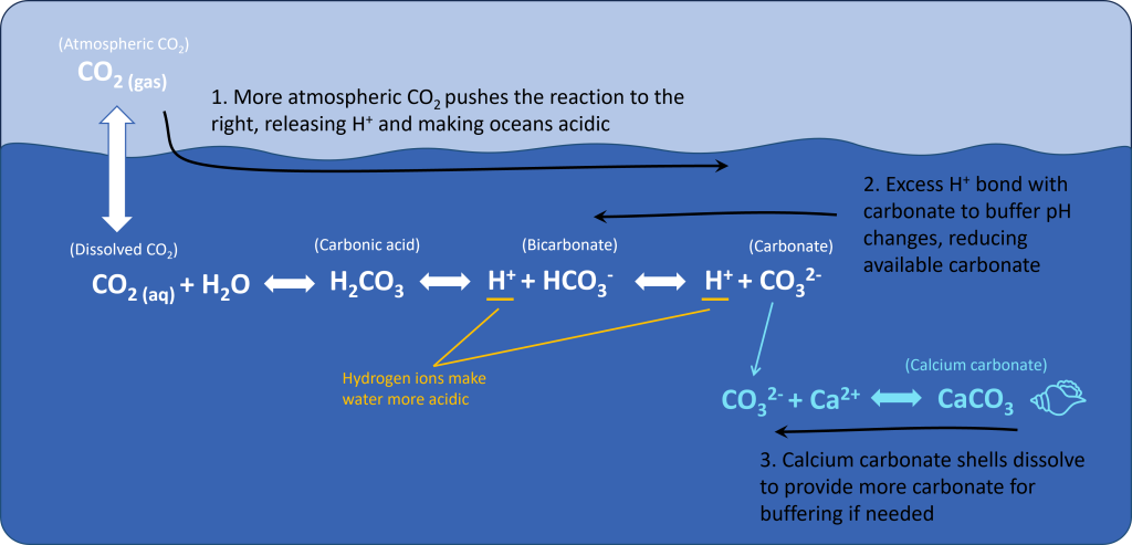
As more and more CO2 molecules are absorbed by the oceans (driving the chemical reactions to the right and creating more H+ in the oceans), the system works to return to equilibrium by bonding more and more carbonate ions with those excess H+ and creating bicarbonate. This results in less carbonate available to bond with calcium to make calcium carbonate. As increasing carbonate is needed to buffer the excess H+, shells will dissolve to return calcium and carbonate into solution where the carbonate will be available to help buffer the ocean’s pH. Organisms that rely on calcium carbonate lose out and cannot build or maintain their shells, skeletons, or other structures.
While technically the extra CO2 absorbed by the oceans has not made oceans acidic (the current pH around 8.1 is still on the basic side of the pH scale), the pH is moving in that direction and will continue to decrease as more CO2 is absorbed. The table below summarizes the projected pH levels by 2100 for the IPCC scenarios. Under the two highest emissions scenarios, ocean pH could drop below 7.8 by 2100, making it more than 150% more acidic than today, and severely impacting marine ecosystems.
| IPCC Scenario | Projected ocean pH by 2100 (approximate) |
| SSP1-1.9 | 8.05 |
| SSP1-2.6 | 8.0 |
| SSP2-4.5 | 7.9 |
| SSP3-7.0 | 7.77 |
| SSP5-8.5 | 7.67 |
The rate of acidification will not be equal everywhere, and as cold water can absorb more gas than warm water, polar regions are more vulnerable to acidification than equatorial regions. But generally, at 1.5°C of warming, ocean acidification is projected to cause a decline in coral reefs by 70-90% and at 2°C of warming, reefs will be close to non-existent.
3.5 Ecosystems
Biome shifts
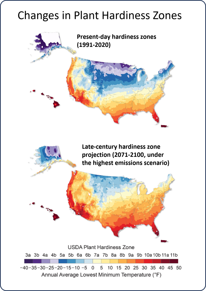
Ecosystems will be profoundly affected by climate change. Polar and marine ecosystems were discussed above in relation to warming temperatures, melting ice sheets, and ocean acidification, but more generally there will be an overall change to climate zones and biomes as the planet warms. This means suitable habitats for plants and animals will shift, creating new challenges for natural ecosystems but also for food production as plant hardiness zones change. The overall effect of the changes is that biomes will move north or south away from the equator towards the poles creating an overall reduction in cold temperature, polar biomes. Across the United States, this means USDA hardiness zones will advance northward. In Minnesota, this will bring a change from the present-day hardiness zones of 3a through 5a, depending on location in the state, to a much warmer 5b through 7a (Figure 3D.3.13).
Invasive Species
Changes to climate also mean changes to invasive species in an area. As air, land, and water temperatures rise it creates new pathways for invasive species to enter an area. Invasive species are those flora or fauna that are not natural to an area. Because these non-native species have no natural predators or other methods to keep their growth in check, they tend to expand rapidly, often out-competing the native species for resources.
Forests
Forests are battling the effects of climate change on several fronts. They must deal with an increased risk from species such as pine beetles and from lack of water. Pine beetles affect pine trees by laying eggs under the bark. As the larva grow and feed it cuts off water and nutrient supplies to the tree, killing it. Pine beetles are responsible for the clusters of dead, red colored pine trees in otherwise healthy pine forests (Figure 3D.3.14, left). While pine beetles are native in some areas, particularly in the mountainous Western U.S., their zone has spread to new areas where they are considered invasive (Figure 3D.3.14, right). This spread has come about because of changes in temperature. Pine beetles cannot survive hard freezes, and so were not historically found at higher elevations where colder winter temperatures kept populations from proliferating. With warmer winters, those cold zones have changed and are now susceptible to pine beetle infestations. In addition, the warmer winters and longer summers have allowed pine beetles to reproduce faster. Pine beetles used to require two years to reproduce and develop, but this process can now occur in a single year.
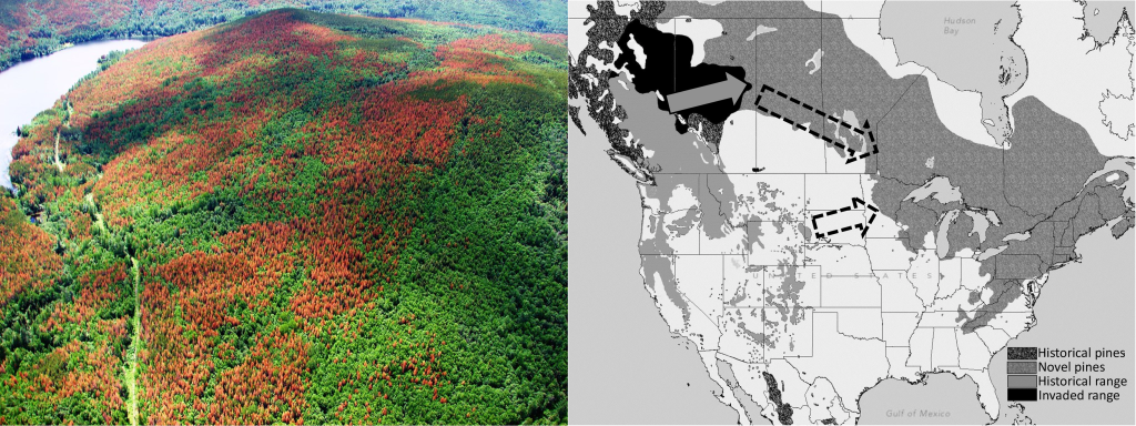
Drought adds another layer to the pine beetle issue. One of the best defenses a tree has against an infestation is by drowning the beetles in a layer of sap. However, as trees dry out, they can no longer produce sap as easily, decreasing their ability to fight off pine beetles.
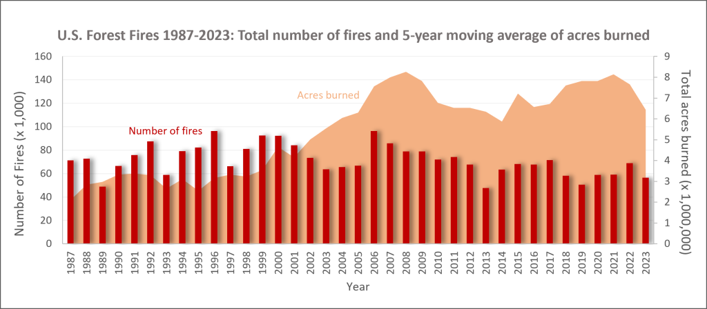
Drought and unhealthy forests, due to things like pine beetle infections, both contribute to increased risk of forest fires. The longer spring and summers have extended the length of the fire season and increased temperatures, decreased spring snowmelt, and decreased precipitation, particularly in the Western U.S., have worsened drought conditions. U.S. federal fire agencies began using the current tracking process for recording wildfires starting in 1983, and since that time, the total number of forest fires has gone up and down but stayed relatively consistent but the number of large fires, and therefore the number of acres burned, has steadily increased (Figure 3D.3.15). Climate models project this trend will continue, with more large fires burning larger areas of land.
3.5 Human Health
The future climate is projected to hold more extreme weather events (heat waves, strong storms, floods, and droughts). This will affect the availability of clean food and water, disrupt communication and emergency services, and impact health care. As discussed, the number of high heat days and heat waves will increase leading to more heat related deaths and putting a strain on the electrical grid as people work to keep themselves cool. Heat, floods, and droughts will all impact agriculture putting a strain on food production and creating food insecurity, which could also lead to wars and other civil conflicts.
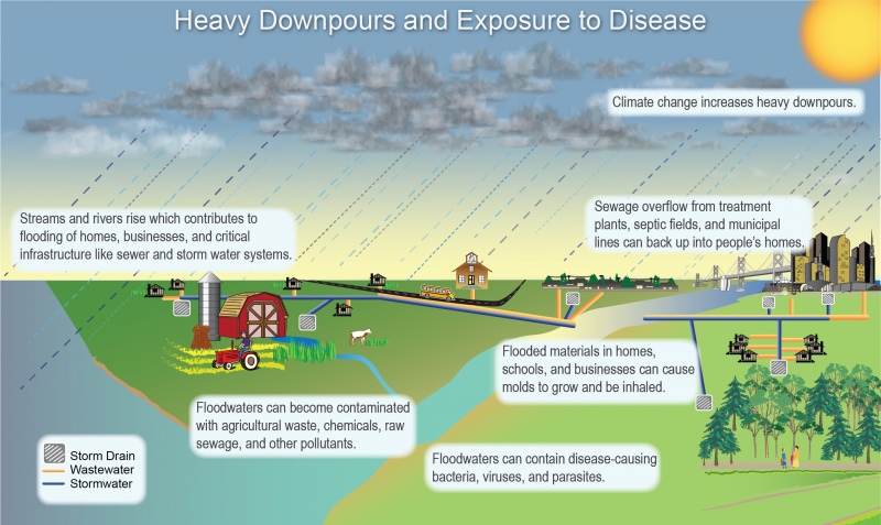
Increased rainfall and flooding can overwhelm existing sewage and water treatment infrastructure. This could create overflows from sewage treatment plants into fresh water sources and increase water-borne parasites such as Cryptosporidium and Giardia that are sometimes found in drinking water. Flooding can also wash chemicals, agricultural waste, and other contaminants from agricultural areas into drinking water sources (Figure 3D.3.16). These can lead to gastrointestinal and other health issues.
Higher air temperatures can increase salmonella and other bacteria-related food poisoning because bacteria grow more rapidly in warm environments. Higher temperatures will also change the locations where various bacterial and viral diseases carried by insects are found (ticks that carry Lyme disease and mosquitoes carrying malaria, dengue fever, West Nile Virus, etc.). Longer summers and warmer winters will increase the length of the season when mosquitoes and other insects carrying these diseases are active.
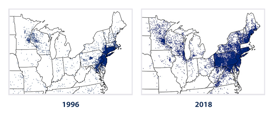
This is shown to be the case with ticks carrying Lyme disease in North America. Climate change has expanded the range of ticks and increased the potential risk of contracting Lyme disease. The life cycle and prevalence of deer ticks (the ticks responsible for spreading Lyme disease), are most active in temperatures above 45°F and with at least 85% humidity. As climate warms, and evaporation and humidity increase, the habitat suitable for ticks carrying Lyme disease (and other illnesses) will spread. This has already been seen across the northern U.S., the area where deer ticks and Lyme disease are most prevalent (Figure 3D.3.17). Shorter winters will also extend the period over which ticks are active in the year, increasing the number of days humans could be exposed to tick-borne illnesses.
Climate change is also affecting air quality in a variety of ways. Ground-level ozone, which is damaging to the lungs and particularly harmful to people with lung health issues, is projected to increase. It is created through a reaction between sunlight and nitrogen oxides, which are emitted from burning fossil fuels. Particulate matter will also increase as droughts dry out the landscape and lead to more windblown dust. Increased wildfires will create more smoke and ash and longer springs and summers will lead to the production of more pollen. All of these changes add to existing air pollution and create new or worsen existing health problems like respiratory issues and heart problems.
Climate change will not only affect physical health, it will also affect mental health. Hotter temperatures are closely linked with increases in violence as people become more irritable and easily triggered under warmer conditions. The added stress of dealing with increasingly frequent climate-induced disasters such as heatwaves, diseases, storms, flooding, food insecurity, etc. can lead to PTSD and create or worsen other mental health issues such as depression and anxiety.
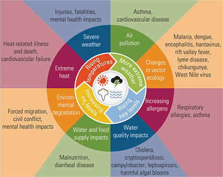
The infographic below summarizes how climate change impacts human health (Figure 3D.3.18)
Climate and Environmental Justice and Equity
The impacts of climate change will not be felt equally everywhere. In part this is a function of climate itself not changing in the same way everywhere, but the larger issue is because not everywhere or everyone has the same ability to deal with the impacts of climate change. This is true at various scales with richer, more developed nations having an advantage over less wealthy, less developed nations but also holds true within a country where wealthier cities or even neighborhoods will be impacted less. This is of particular importance related to human health. Many socially vulnerable groups live in industrial or urban areas with high levels of air pollution. In fact, Black and African American individuals are 34% more likely than non-Black individuals to live in areas with the highest projected increases in childhood asthma due to climate-related changes in particulate matter. Air quality impacts will also affect certain populations more based on jobs. Farm workers, construction workers, landscapers, and other outdoor workers will be more vulnerable to air quality impacts due to increased exposure.
Both rural and urban low-income populations are more likely to live in older buildings or buildings that are in poor condition. These buildings may not be well sealed, increasing exposure to outdoor allergens and pollutants. These buildings are also more likely to take damage during extreme weather like storms and floods leading to the growth of mold, bacteria, and other indoor air contaminants.
Vulnerable communities may have reduced access to or ability to afford measures such as air conditioning to stay cool during heatwaves. This greatly increases the risk of heat related illnesses and death. The populations that are most vulnerable during heatwaves are low-income earners, the sick, the elderly, and infants.
Keeping warming to 1.5°C will reduce the number of people impacted by climate-related health risks. A rise of 2°C could cause several hundred million more people to be susceptible to climate-related health impacts.
Check your understanding: Consequences of climate change
Drag and drop the climate change consequence from the right hand side of the chart into either the appropriate column to indicate if that consequence is projected to increase or decrease in the future.
References
IPCC (2021). Climate Change 2022: Impacts, adaptation and Vulnerability. https://www.ipcc.ch/report/ar6/wg2/
Jahn, A., Holland, M. M., & Kay, J. E. (2024). Projections of an ice-free Arctic Ocean. Nature Reviews. Earth & Environment. https://doi.org/10.1038/s43017-023-00515-9
Knutson, T. (2024, April 17). Global Warming and Hurricanes: An Overview of Current Research Results. NOAA Geophysical Fluid Dynamics Laboratory. https://www.gfdl.noaa.gov/global-warming-and-hurricanes/
Buis, A. (2020, October 12). A degree of concern: Why global temperatures matter. NASA Global Climate Change Website. https://climate.nasa.gov/news/2865/a-degree-of-concern-why-global-temperatures-matter/
National Snow and Ice Data Center (2018, January 3). Arctic Sea Ice news and Analysis. https://nsidc.org/arcticseaicenews/2018/01/
Rosenberger, D. W., Venette, R. C., Maddox, M. P., & Aukema, B. H. (2017). Colonization behaviors of mountain pine beetle on novel hosts: Implications for range expansion into northeastern North America. PloS One, 12(5), e0176269. https://doi.org/10.1371/journal.pone.0176269
Sung, H. M., Kim, J., Shim, S., Seo, J., Kwon, S., Sun, M., Moon, H., Lee, J., Lim, Y. C., Boo, K., Kim, Y., Lee, J., Lee, J., Kim, J., Marzin, C., & Byun, Y. (2021). Climate change projection in the Twenty-First Century simulated by NIMS-KMA CMIP6 model based on new GHGs concentration pathways. Asia-Pacific Journal of Atmospheric Sciences, 57(4), 851–862. https://doi.org/10.1007/s13143-021-00225-6
Tebaldi, C., Debeire, K., Eyring, V., Fischer, E. M., Fyfe, J. C., Friedlingstein, P., Knutti, R., Lowe, J., O’Neill, B. C., Sanderson, B. M., Van Vuuren, D., Riahi, K., Meinshausen, M., Nicholls, Z., Tokarska, K., Hurtt, G., Kriegler, E., Lamarque, J., Meehl, G. A., . . . Ziehn, T. (2021). Climate model projections from the Scenario Model Intercomparison Project (ScenarioMIP) of CMIP6. Earth System Dynamics, 12(1), 253–293. https://doi.org/10.5194/esd-12-253-2021
United States Environmental Protection Agency (2023, November 1) Climate change indicators: Lyme Disease. https://www.epa.gov/climate-indicators/climate-change-indicators-lyme-disease

_-_annually.svg)