4. Late Cenozoic Ice Age
4.1 Causes of Glaciation
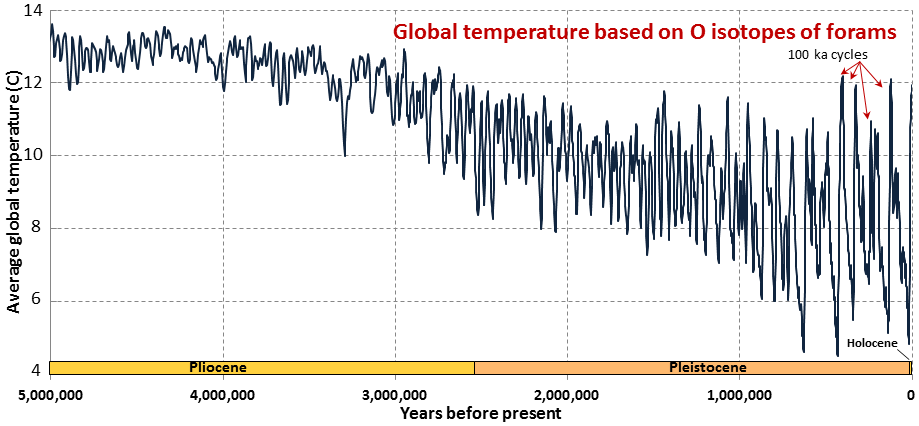
The greenhouse conditions that began following the end of the Late Paleozoic Ice Age and peaked during the Eocene Epoch of the Early Cenozoic Era lasted until 34 million years ago, when the planet went back into an ice age at the start of the Oligocene Epoch. This ice age has persisted through the present day (Figure 3B.4.1). This began with the growth of ice sheets on Antarctica around 34 Ma followed by growth of Northern Hemisphere ice sheets around 3 Ma. Since the onset of the current ice age, the extent of continental ice sheets has waxed and waned through glacial and interglacial cycles. In the current interglacial cycle, only the Antarctic and Greenland ice sheets are still present.
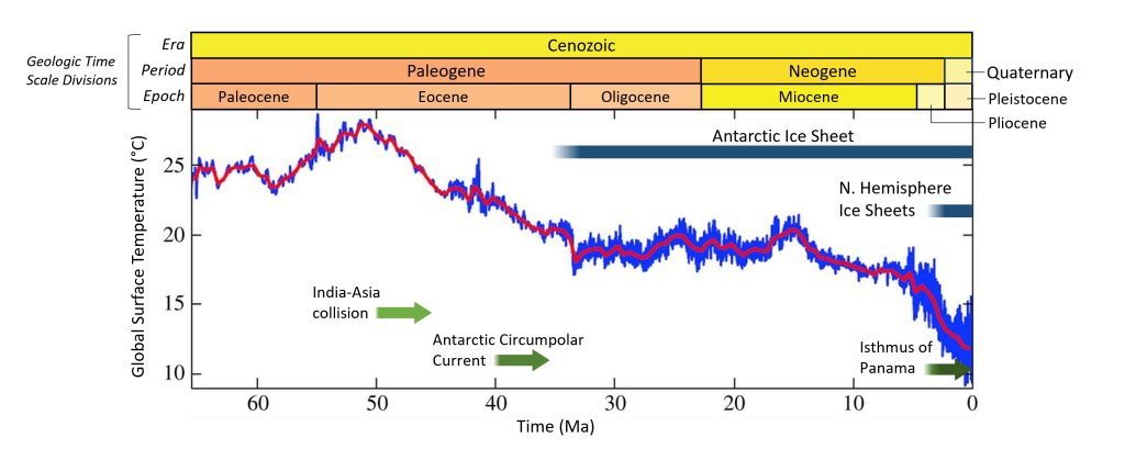
The cooling of the planet from the warm climate of the Early Eocene is attributed to a series of plate tectonic events. The collision of the Indian Plate with the Eurasian Plate began the process of Himalayan mountain building around 50 Ma. The rapid uplift of these mountains and formation of the high landscape of the Himalayan-Tibetan Plateau increased rates of weathering and erosion pulling CO2 out of the atmosphere and initiating long term cooling.
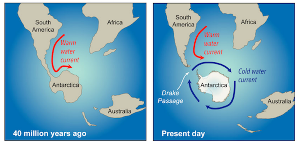
Around 40 Ma, plate motions widened the narrow gap between South America and Antarctica opening the Drake Passage. Prior to this, the arm of land connecting South America and Antarctica allowed warm ocean currents to carry heat from the equator to Antarctica, but when the gap opened up, a new cold-water current, the Antarctic Circumpolar Current, formed (Figure 3B.4.2). This current flows in a continuous loop around Antarctica and blocks warm water from reaching Antarctica. In the already cooling climate, the isolation of Antarctica from warm water currents cooled the southern polar region further, allowing ice sheets to grow by about 34 Ma, marking the onset of the Late Cenozoic Ice Age.
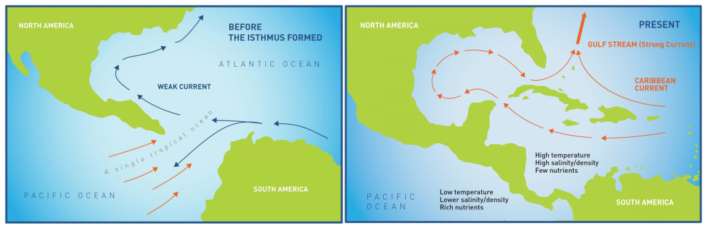
Following the start of Antarctic glaciation, temperatures leveled off, remaining around 18-20 °C throughout the Oligocene and Early Miocene (Figure 3B.4.1). During this time, Antarctic ice sheets waned but did not melt away altogether and the Northern Hemisphere remained ice free. Ongoing plate tectonics forced another change to climate by creating the Isthmus of Panama. This is the narrow strip of land that separates the Caribbean Sea from the Pacific Ocean in the region of the present-day country of Panama. It was created through volcanism associated with eastward subduction under the Caribbean Plate. Prior to the Isthmus of Panama, the Central American Seaway allowed movement of warm tropical water between the Pacific and Caribbean through this area. The closure of this seaway 3-5 million years ago forced ocean currents into a new path intensifying the warm Gulf Stream current, the shallow current that carries heat and moisture north along the coast of eastern North America before heading across the North Atlantic to Northern Europe (Figure 3B.4.3). Cooling and evaporation of this water in the North Atlantic strengthened thermohaline circulation and introduced extra moisture to the Arctic region. This influx of moisture provided the necessary water to feed ice sheet growth in the Northern Hemisphere beginning about 3 million years ago in the Late Pliocene.
The Pleistocene Epoch, the time period from 2.58 Ma to about 12,000 years ago, is characterized by intense glaciation across the Northern Hemisphere, with average global temperatures being 4 to 10 °C (about 8-20 F) cooler than present day. This time period is known as the Pleistocene Glaciation, the Quaternary Glaciation, or simply the Ice Age. It is the time of woolly mammoths and saber tooth tigers popularized in movies.
As the most recent time period of extensive glaciation, this cold period also has the best-preserved record of temperature fluctuations. Through the study of ice cores and seafloor sediments a clear pattern of glacial-interglacial cycles has been identified throughout this time frame (Figure 3B.4.4). The high to low temperature variations correspond to contraction and expansion of ice sheets, respectively, with major fluctuations occurring on a 100,000-year cycle. This time interval is a result of Milankovitch Cycle orbital changes. Changing solar irradiance from the Milankovitch Cycles drove the glacial-interglacial cycles in the cooler climate brought on by the earlier plate tectonic events.

4.2 Effects of the Pleistocene Glaciation
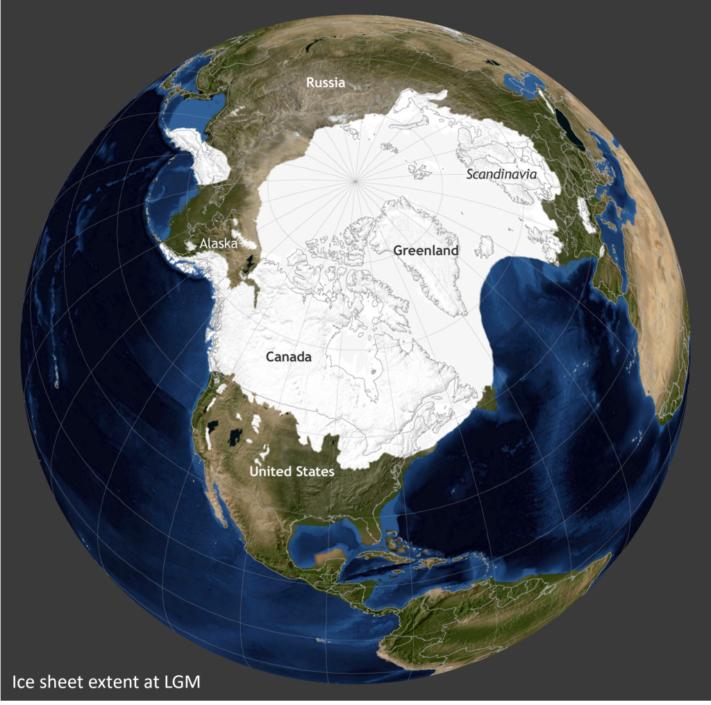
Glaciation reached a peak about 20,000 years ago during the Last Glacial Maximum (LGM). At this time ice sheets were at their largest, covering sizable portions of North America and Northern Europe (Figure 3B.4.5). The water to grow ice sheets was supplied from the oceans, so as ice sheets grew sea level dropped. Sea level was lower by 125 m (over 400 ft) during LGM, exposing land areas that flooded once the ice sheets receded again. On Figure 3B.4.5 the present-day coastline is outlined in white for comparison with ocean levels during the LGM.
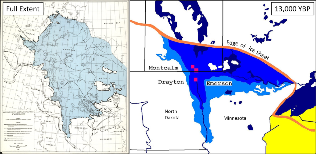
At the end of the Pleistocene Glaciation, the climate was warming and entering the current interglacial cycle in the Late Cenozoic Ice Age. As the ice sheets retreated, they left massive lakes of glacial meltwater on the landscape. Lakes formed in this way are termed proglacial lakes. A significant one of these in North America was Lake Agassiz, which covered most of Manitoba and western Ontario in Canada and covered a major portion of northern Minnesota with a long arm that extended along the Minnesota-North Dakota border in the present-day location of the Red River Valley (Figure 3B.4.7, left). At its maximum, it was the largest freshwater lake to have ever existed on the planet, with a volume greater than all of the Great Lakes combined. Lake Agassiz existed because this area of land drains north into Hudson Bay, but the slow retreat of the ice sheet kept the outlet to Hudson Bay blocked (Figure 3B.4.7, right). The meltwater had nowhere to go other than to pool into a massive lake on the edge of a retreating ice sheet. As the edge of the ice sheet slowly retreated north, the location of Lake Agassiz shifted north as well until finally an outlet to Hudson Bay was established and the lake water drained into the Bay. Present day remnants of Lake Agassiz include Red Lake, Rainy Lake, and Lake of the Woods in Minnesota, Lake Manitoba, Lake Winnipeg, and Lake Winnipegosis in Manitoba.
Minnesota Connection: Flooding in the Red River Valley
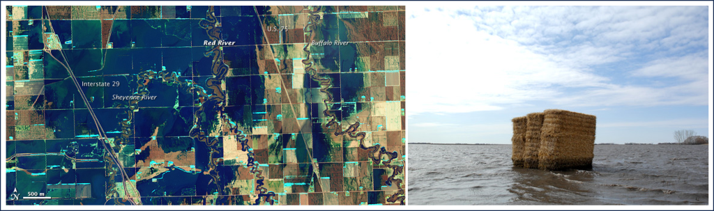
Flooding along the Red River Valley, the area situated on the North Dakota-Minnesota border and extending north into Manitoba, is a yearly occurrence. The propensity for flooding in this region is a direct result of the Pleistocene Glaciation.
Glacial ice is dirty, carrying lots of clay, silt, sand, and gravel. As the ice flows over the landscape, it essentially behaves like a giant piece of sandpaper, scraping the landscape flat. Lake Agassiz pooled over this already flat landscape contributing a layer of lake floor sediments rich in clay and silt. As the lake emptied off of the landscape, the Red River was left to drain this area. The Red River flows north along the Minnesota-North Dakota border through what was the southern arm of Lake Agassiz; a landscape that is both very flat and very rich in clay sediments. Almost every year during the spring, snow meltwater raises the river levels and the Red River Valley floods. With a flat landscape and clay rich sediment, the flood waters do not have anywhere to go. The flatness means water can spread quite far and then pool on the landscape as there is no slope to encourage it to flow back into the river channel (Figure 3B.4.8). In addition, the clay rich soils have low permeability making it hard for floodwater to infiltrate into groundwater.
These are only a few of the many landscape effects that occurred as a result of Pleistocene Glaciation both in Minnesota and across the planet.
Check your understanding: Late Cenozoic Ice Age
References
Ehlers, J., & Gibbard, P. L. (2007). The extent and chronology of Cenozoic Global Glaciation. Quaternary International, 164–165, 6–20. https://doi.org/10.1016/j.quaint.2006.10.008
Hansen, J. E., Sato, M., Russell, G. L., & Kharecha, P. (2013). Climate sensitivity, sea level and atmospheric carbon dioxide. Philosophical Transactions of the Royal Society A, 371(2001), 20120294. https://doi.org/10.1098/rsta.2012.0294
Haug, G. H., & Tiedemann, R. (1998). Effect of the formation of the Isthmus of Panama on Atlantic Ocean thermohaline circulation. Nature, 393(6686), 673–676. https://doi.org/10.1038/31447
Hayashi, T., Yamanaka, T., Hikasa, Y., Sato, M., Kuwahara, Y., & Ohno, M. (2020). Latest Pliocene Northern Hemisphere glaciation amplified by intensified Atlantic meridional overturning circulation. Communications Earth & Environment, 1(1). https://doi.org/10.1038/s43247-020-00023-4
Lisiecki, L. E., and M. E. Raymo (2005), A Pliocene-Pleistocene stack of 57 globally distributed benthic d18O records, Paleoceanography, 20, PA1003, doi:10.1029/2004PA001071
Livermore, R., Hillenbrand, C., Meredith, M. P., & Eagles, G. (2007). Drake Passage and Cenozoic climate: An open and shut case? Geochemistry Geophysics Geosystems, 8(1). https://doi.org/10.1029/2005gc001224
Pringle. H. (2017, March 8). What happens when an archaeologist challenges mainstream scientific thinking? Hakai Magazine. https://www.smithsonianmag.com/science-nature/jacques-cinq-mars-bluefish-caves-scientific-progress-180962410/
Teller, J. T., L. H. Thorleifson, L. A. Dredge, H. C. Hobbs and B. T. Schreiner. Maximum Extent and Major Features of Lake Agassiz [map]. 1:3,000,000. In: Geological Association of Canada. Special Paper 26. [Ottawa]: Geological Association of Canada, 1983
Zachos, J. C., Pagani, M., Sloan, L. C., Thomas, E., & Billups, K. (2001). Trends, Rhythms, and Aberrations in Global Climate 65 Ma to present. Science, 292(5517), 686–693. https://doi.org/10.1126/science.1059412
Zachos, J. C., Dickens, G. R., & Zeebe, R. E. (2008). An early Cenozoic perspective on greenhouse warming and carbon-cycle dynamics. Nature, 451(7176), 279–283. https://doi.org/10.1038/nature06588
