5. Measuring Past Climates

Information about Earth’s climate in the past, or paleoclimate, is determined using multiple types of data. Some of these data can be measured directly using instruments such as thermometers to measure temperature, rain gauges to measure precipitation amounts, or satellite imagery to measure the extent of ice sheets or changes in coastline locations. If these measurements are taken and recorded consistently, a very complete record of climate is created through these direct data. Direct data of global climate have been collected since about 1850. To reconstruct climatic conditions further in the past, indirect records of the climate must be used. These indirect records are known as proxy data. They are physical or chemical characteristics of the environment preserved in the geologic record and stand in for direct data to understand climate in the past. Proxy data are used to understand the conditions during the greenhouse and icehouse intervals discussed previously. Direct data are collected today to understand current climate changes.

There are many types of proxy data used to understand paleoclimate. Some of these data can inform understanding of climate many millions of years ago, while others are useful only over the most recent hundreds to thousands of years. A number of proxy data types are discussed below in order of those that are useful only for the relatively recent past through those that can be used for paleoclimate millions of years ago.

5.1 Tree Rings

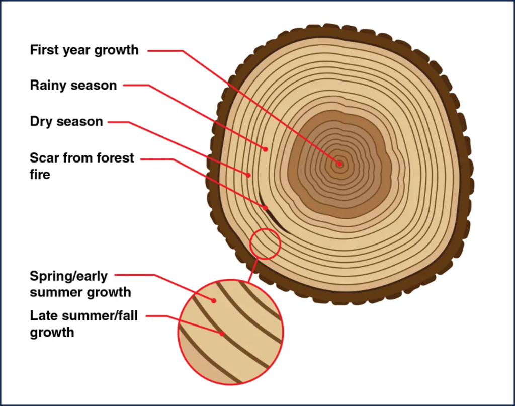
Trees grow by creating new layers of cells on the outside of the tree making tree trunks and branches wider each year. This creates a new ring of material that marks a full year of growth (Figure 3B.5.1). Climatic conditions influence the width, density, and isotopic composition of these growth rings. For example, if a tree species is particularly dependent on a certain condition such as temperature or rainfall during its growing season, it will create wider rings when optimal conditions are present but narrower rings when growing conditions are not as good. In this way, climatic information can be gained by studying tree rings patterns. Tree rings can be used to interpret climatic information going back hundreds to thousands of years.

5.2 Pollen

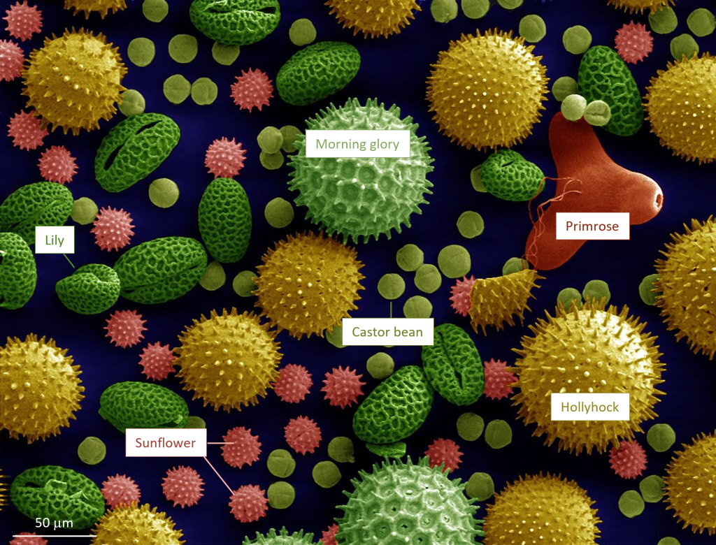
Pollen, that powdery substance produced by flowering plants and seed plants like conifers, has distinctive shapes that allow it to be used to identify the plant it came from (Figure 3B.5.2). Pollen becomes incorporated and preserved in sediment layers at the bottom of a pond, lake, or ocean and analysis of the pollen grains tells scientists what type of plants were growing when that sediment layer was deposited. As plants have specific ranges of climatic zones in which they are adapted to live, the mix of pollens preserved in the sediment provides information about the climate at that time. Pollen records can be used to interpret paleoclimate going back hundreds of thousands to even a few million years.

5.3 Isotope Analyses

As temperature changes, so does the ratio of certain isotopes in the air, rain, and ocean water. This isotopic signal gets preserved in glacial ice, seafloor sediments, and cave deposits. This record can be used to interpret paleoclimate going back hundreds of thousands of years in ice cores to tens of millions of years in seafloor sediments. Many different isotopes are used for this work depending on the geologic material being analyzed, but oxygen isotopes are widely used in all materials.

What are isotopes?

To understand what an isotope is requires understanding the basic structure of an atom. Atoms are the basic, fundamental unit of all matter. They are composed of protons, neutrons, and electrons.

Electrons are the negatively charged particles that orbit around the nucleus of an atom. The addition or loss of electrons changes the charge of an atom, creating ions. Adding electrons creates a negative charge while losing electrons creates a positive charge.

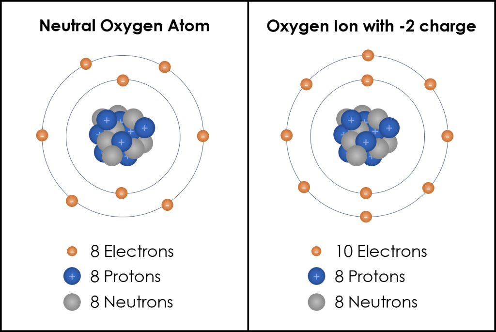
The center, or nucleus, of the atom contains protons and neutrons. Protons are the positively charged particles in an atom. The number of protons contained in the nucleus determines what element the atom is. For example, an atom of oxygen will always have 8 protons and a carbon atom will always have 6 protons. When an atom is neutral, the number of protons (positive charge) equals the number of electrons (negative charge). So, for oxygen, this is when there are 8 electrons orbiting to balance the 8 protons in the nucleus (Figure 3B.5.3, left). If the oxygen atom gains 2 electrons, now there are two extra negative charges compared to the 8 positive charges and this creates an oxygen ion with a charge of negative two (Figure 3B.5.3, right).

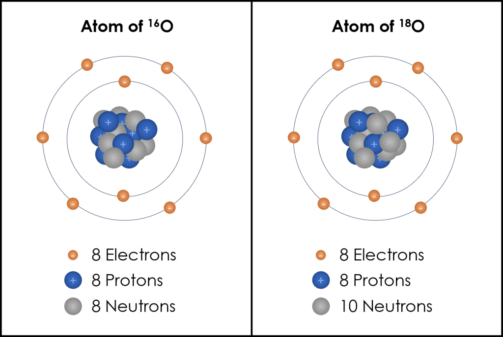
Neutrons are the other particles contained in the nucleus with the protons and they do not have a charge; they are neutral. Isotopes are atoms of the same element that have a different number of neutrons. In other words, isotopes of an atom have the same number of protons but a different number of neutrons. The mass of an atom is determined by the number of protons and neutrons (i.e., the mass of the nucleus) as electrons are much smaller and their mass is negligible when compared to that of the nucleus. Therefore, the different number of neutrons in an isotope of the same element means isotopes have different masses and these mass differences are used to name the isotopes. Oxygen has two main isotopes: ¹⁶O and ¹⁸O (pronounced sixteen O or sixteen oxygen and eighteen O or eighteen oxygen), where the number is the mass of the atom. In ¹⁶O, there are 8 protons and 8 neutrons (8 + 8 = 16), and in ¹⁸O there are 8 protons (remember, the number of protons is what makes it an oxygen!) and 10 neutrons (8 + 10 = 18) (Figure 3B.5.4).

Generally one isotope is in much higher abundance than the others. In the case of oxygen, most oxygen is in the form of ¹⁶O (about 99.75% of all oxygen atoms) and only a small portion is as ¹⁸O (0.2%). The remaining even smaller portion is a third isotope of oxygen, ¹⁷O.

Check your understanding: Basic chemistry of isotopes

Physical, chemical, and biological processes change the ratio of the heavier ¹⁸O to the lighter ¹⁶O in the atmosphere, rainwater, seawater, etc. The natural abundance of the lighter ¹⁶O is much higher, so the total amount of this lighter isotope will always be much higher than that of the heavier ¹⁸O, but processes can slightly increase or slightly decrease the abundance of the heavier oxygen making the overall ratio of ¹⁸O to ¹⁶O slightly higher or slightly lower, respectively. This makes water formed with higher or lower ratios of ¹⁸O to ¹⁶O literally heavier or lighter, respectively. How processes change the isotopic ratio of oxygen and how much that ratio changes are well known and well correlated to temperature conditions. The general term used for the change in ratio of isotopes due to various processes is called isotopic fractionation because the ratio or fraction of isotopes changes.

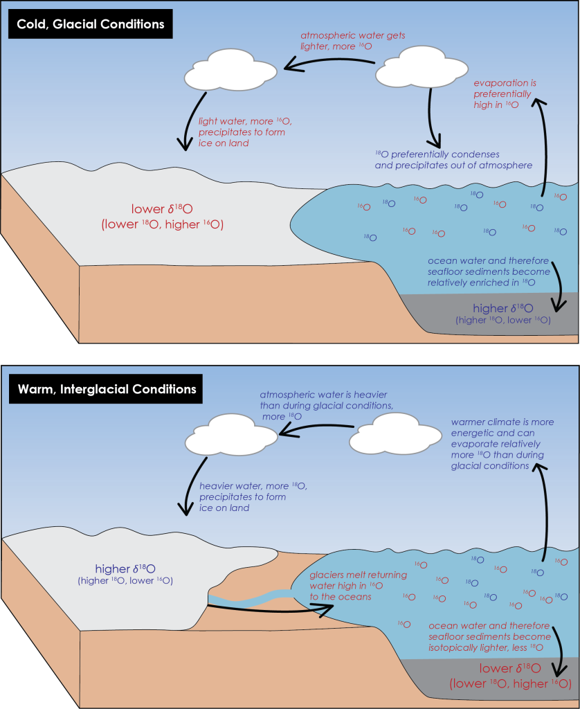
While isotopic fractionation of oxygen can be complex in detail, Figure 3B.5.5 below provides a simplified overview of how precipitation and ocean water become heavier or lighter as a result of isotopic fractionation in different climate conditions. It requires less energy and is easier to evaporate lighter isotopes, as a result they preferentially evaporate first from the oceans. In addition, as water condenses into rain in the atmosphere, heavier isotopes condense first, falling as rainwater and being returned to the oceans, while lighter isotopes remain as gas in the atmosphere to be transported. During glacial time periods, evaporation and condensation work together to cause oceans to become enriched in heavier isotopes, ¹⁸O, while the air mass that transports towards the poles and eventually condenses to make snow and then glacial ice is reduced in heavier isotopes and enriched in lighter ¹⁶O isotopes. Organisms in the oceans take up oceanic oxygen and use this to build calcium carbonate shells. Their shells record the ratio of heavy to light oxygen that is present in ocean water, so during glacial times, their shells are also enriched in heavy oxygen. As these organisms die, their shells sink to the ocean floor and become part of the sediment layers there (microscopic foraminifera are important components making up seafloor sediments). These sediments get solidified into rocks and in this way the isotopic record of ocean water, and therefore climate, gets preserved. During colder interglacial conditions, seafloor sediments show an increase in the ratio of ¹⁸O to ¹⁶O, i.e., they have more heavy oxygen, while glacial ice is depleted in heavy oxygen/enriched in light oxygen, showing a decrease in the ratio of ¹⁸O to ¹⁶O (Figure 3B.5.5, top).

This changes during warmer climates. When temperatures rise, glacial ice melts returning water enriched in light oxygen back to the oceans. This decreases the ¹⁸O to ¹⁶O ratio in ocean water, making oceans and therefore seafloor sediments lighter than during cold climates. Glacial ice can still be created during warmer climates and because the entire system is warmer and has more energy to evaporate and transport water, ice made during this time has more heavy oxygen, a higher ¹⁸O to ¹⁶O ratio, than during cold climates (Figure 3B.5.5, bottom).

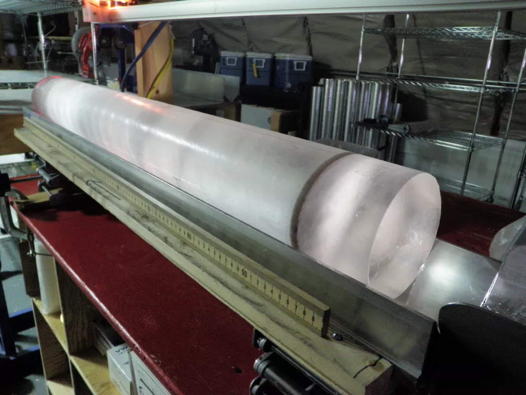
Oxygen isotopes measured from ice cores provide climatic information going back many hundreds of thousands of years. Isotope records from seafloor sediments can go much further back in time, providing climatic information for the past tens of millions of years. Scientists drill into the ice or seafloor sediments to collect a long core of material (Figure 3B.5.6). From this, samples are taken at small intervals along the core and analyzed to determine the age of the core at that location and to collect climate proxy data. Only small portions of the core are sampled, so most of the core remains intact and is stored allowing for more analyses to be conducted in the future.

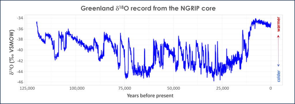
Temperatures are calculated from isotope ratios using well established and tested mathematical conversions. The graph in Figure 3B.5.7 shows the oxygen isotope data from one of the ice cores, labeled NGRIP, drilled in Greenland. Note the y-axis label for the isotope data is δ¹⁸O. This is called delta notation (δ is the lowercase Greek letter delta), and it represents that the axis values are not absolute measurements of the heavy to light isotope ratio, but rather showing how much that isotope ratio has changed relative to a standard isotope ratio. In the case of oxygen isotopes, the standard ratio being measured against is Vienna Standard Mean Ocean Water (VSMOW). This change is expressed in units of ‰ or per mil, which is parts per thousand in the same way that  %, or percent, is parts per hundred. Higher delta values (less negative) indicate warmer temperatures and lower delta values (more negative) indicate colder temperatures.

5.4 Greenhouse Gas Analyses

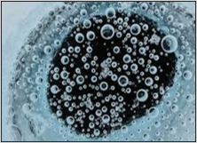
Another proxy set of proxy data are found by analyzing gas bubbles that are preserved at depth in ice cores. As snow layers are compacted into glacial ice, air bubbles containing atmospheric air get trapped in the ice layers. These bubbles preserve the concentration of atmospheric gases at the time glacial ice formed (Figure 3B.5.8).

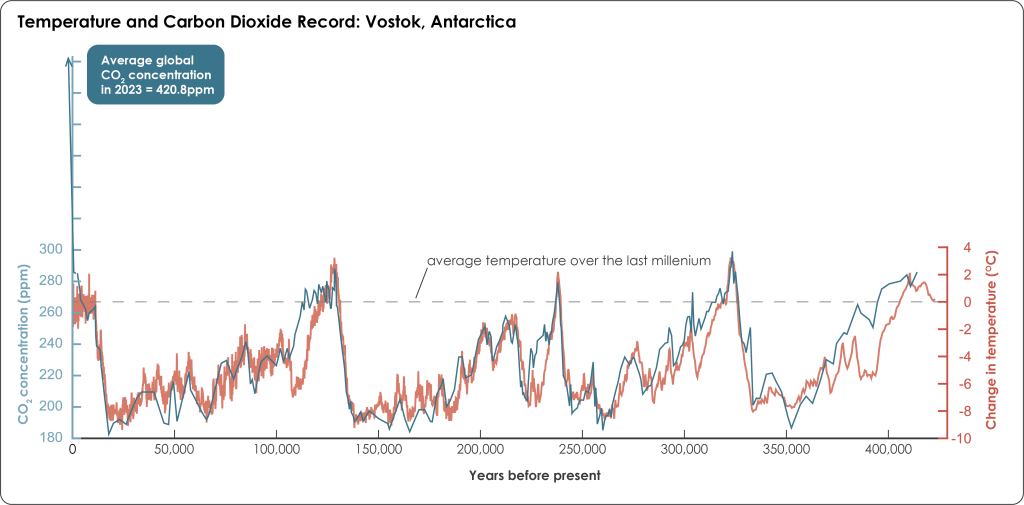
The air bubbles are extracted by melting, crushing, or grating the ice in a vacuum and the concentration of CO₂, methane, and other greenhouse gases are measured giving a record of these gas concentrations in the past. Greenhouse gas concentrations cannot be used to directly calculate temperature the way isotopic data can, but because the chemistry of greenhouse gases and the greenhouse effect are well understood, gas concentrations are useful for examining fluctuations from warmer to colder climates(Figure 3B.5.9).

References

Petit, J., Jouzel, J., Raynaud, D., Barkov, N. I., Barnola, J., Basile, I., Bender, M. L., Chappellaz, J., Davis, M. E., Delaygue, G., Delmotte, M., Kotlyakov, V. M., Legrand, M., Lipenkov, V. Y., Lorius, C., Pépin, L., Ritz, C., Saltzman, E. S., & Stiévenard, M. (1999). Climate and atmospheric history of the past 420,000 years from the Vostok ice core, Antarctica. Nature, 399(6735), 429–436. https://doi.org/10.1038/20859