8 Chap 2 Sample Exercise
Chap 2 Sample Exercise Including Goal Seek
Running your own lawn care business can be an excellent way to make money over the summer while on break from college. It can also be a way to supplement your existing income for the purpose of saving money for retirement or for a college fund. However, managing the costs of the business will be critical in order for it to be a profitable venture. In this exercise you will create a simple financial plan for a lawn care business by using the skills covered in this chapter. Begin this exercise by opening the file named Chapter 2 CiP Exercise 1.
Click cell C5 in the Annual Plan worksheet.
Enter a formula that calculates the average price per lawn cut. Type an equal sign (=), then click cell B3. Type the asterisk symbol (*) for multiplication, then click cell B4. Press the ENTER key.
Click cell C8 in the Annual Plan worksheet.
Enter a formula that calculates the total number of lawns that will be cut during the year. Type an equal sign (=), then click cell B6. Type the asterisk symbol (*) for multiplication, then click cell B7. Press the ENTER key.
Click cell D9 in the Annual Plan worksheet.
Enter a formula that calculates the total sales for the plan. Type an equal sign (=), then click cell C5. Type the asterisk symbol (*) for multiplication, then click cell C8. Press the ENTER key.
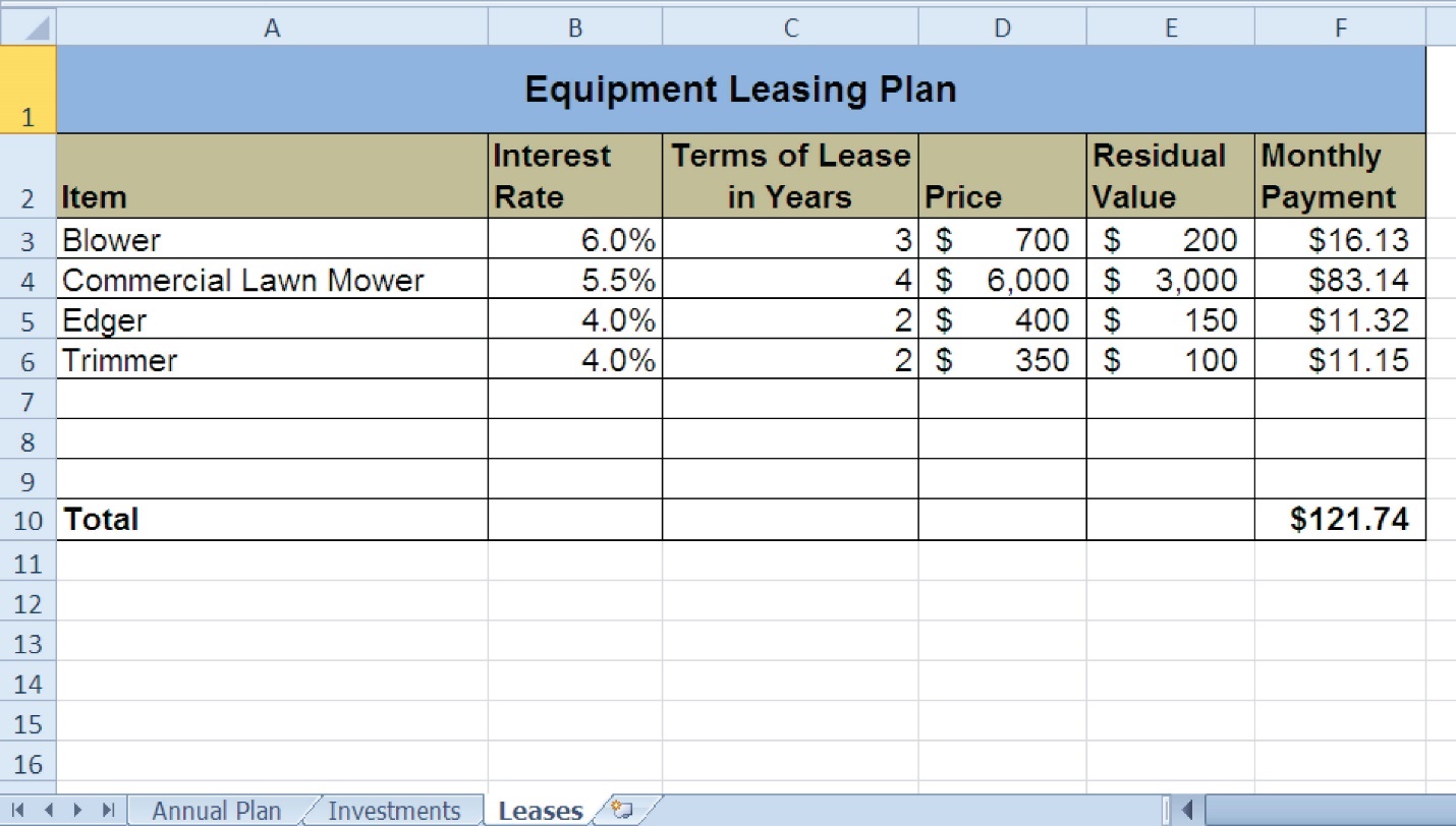
Click cell F3 in the Leases worksheet. The PMT function will be used to calculate the monthly lease payment for the first item. For many businesses, leasing (or renting) equipment is a more favorable option than purchasing equipment because it requires far less cash. This enables you to begin a business such as a lawn care business without having to put up a lot of money to buy equipment.
Type an equal sign (=) followed by the function name PMT and an open parenthesis ((). Define the arguments of the function as follows:
Rate: Click cell B3, type a forward slash (/) for division, type the number 12, and type a comma. Since we are calculating monthly payments, the annual interest rate must be converted to a monthly interest rate.
Nper: Click cell C3, type an asterisk (*) for multiplication, type the number 12, and type a comma. Similar to the Rate argument, the terms of the lease must be converted to months since we are calculating monthly payments.
Pv: Type a minus sign (−), click cell D3, and type a comma. Remember that this argument must always be preceded by a minus sign.
Fv: Click cell E3 and type a comma.
Type: Type the number 1, type a closing parenthesis ()), and press the ENTER key. We will assume the lease payments will be made at the beginning of each month, which requires that this argument be defined with a value of 1.
Copy the PMT function in cell F3 and paste it into the range F4:F6.
Click cell F10 in the Leases worksheet. A SUM function will be added to calculate the total for the monthly lease payments.
Type an equal sign (=) followed by the word SUM and an open parenthesis ((). Highlight the range F3:F9, type a closing parenthesis ()), and press the ENTER key. You will notice that blank rows were included in this range for the SUM function. If other items are added to the worksheet, they will be included in the output of the SUM function.
Highlight the range A2:F6 on the Leases worksheet. The data in this range will be sorted.
Click the Sort button in the Data tab of the Ribbon. In the Sort dialog box, select the Interest Rate option in the “Sort by” drop-down box. Select Largest to Smallest for the sort order. Then, click the Add Level button on the Sort dialog box. Select the Price option in the “Then by” drop-down box. Select Largest to Smallest for the sort order. Click the OK button in the Sort dialog box.
Click cell B11 on the Annual Plan worksheet. The monthly lease payments that are calculated in the Lease worksheet will be displayed in this cell.
Type an equal sign (=). Click the Leases worksheet tab, click cell F10, and press the ENTER key.
Click cell C12 on the Annual Plan worksheet.
Type an equal sign (=) and click cell B11. Type an asterisk (*), type the number 12, and press the ENTER key. This formula calculates the annual lease payments.
Format the output of the formula in cell C12 so the decimal places are reduced to zero.
Click cell C14 on the Annual Plan worksheet.
Type an equal sign (=) and click cell B13. Type an asterisk (*), click cell C8, and press the ENTER key.
Click cell D16 on the Annual Plan worksheet.
Type an equal sign (=) followed by the word SUM and an open parenthesis ((). Highlight the range C11:C15, type a closing parenthesis ()), and press the ENTER key. This SUM function adds the total expenses for the business.
Click cell D17 on the Annual Plan worksheet.
Type an equal sign (=). Click cell D9, type a minus sign (–), click cell D16, and press the ENTER key. This formula calculates the annual profit for the business.
Click cell B10 on the Investments worksheet.
Type an equal sign (=) followed by the word COUNT and an open parenthesis ((). Highlight the range B3:B8, type a closing parenthesis ()), and press the ENTER key. This function counts the number of investments that currently have a balance. Notice that additional blank rows were included in the range for this function. The function output will automatically change if any new investments are added to the worksheet.
Click cell D3 on the Investments worksheet.
Type an equal sign (=). Click the Annual Plan worksheet tab. Click cell D17 and type a forward slash (/) for division. Click the Investments worksheet tab. Click cell B10 and press the ENTER key. This formula divides the profit calculated on the Annual Plan worksheet by the number of investments in the Investments worksheet. We will assume that the profits from this business will be invested evenly among the funds listed in Column A of the Investments worksheet.
Before copying and pasting the formula created in step 28, absolute references must be added to the cell locations in the formula. Double click cell D3 on the Investments worksheet. Place the mouse pointer in front of D17 in the formula and click. Press the F4 key on your keyboard. Place the mouse pointer in front of cell B10 in the formula and click. Press the F4 key on your keyboard. Press the ENTER key.
Copy cell D3 and paste it into cells D4 and D5.
Click cell E3 on the Investments worksheet. The future value function will be added to project the total growth of the investments listed in Column A. We will assume that the business will be able to consistently generate the profit, which will be invested evenly in the funds every year.
Type an equal sign (=) followed by the function name FV and an open parenthesis ((). Define the arguments of the function as follows:
Rate: Click cell C3 and type a comma. This is the expected growth rate of the first fund.
Nper: Type the number 10 and then type a comma. We will project the growth of these investments in 10 years.
Pmt: Type a minus sign (−), click cell D3, and type a comma. Remember that this argument must always be preceded by a minus sign. We are assuming that the business will consistently generate the profits calculated in the Annual Plan worksheet and that these profits will be invested evenly into each fund.
Pv: Type a minus sign (–) and click cell B3. Since each fund currently has a balance, we need to add this to the Pv argument of the function. Similar to the Pmt argument, remember that this argument must also be preceded by a minus sign.
Type: Type a closing parenthesis ()) and press the ENTER key. We will assume the investments will be made at the end of each year. Therefore, it is not necessary to define this argument since Excel will assume zero, or end of the period, if it is not defined.
Copy the FV function in cell E3 and paste it into cells E4 and E5.
Click cell B9 on the Investments worksheet.
Type an equal sign (=) followed by the word SUM and an open parenthesis ((). Highlight the range B3:B8, type a closing parenthesis ()), and press the ENTER key. This SUM function adds the current balance for all investments. Blank rows are added to the range for the function so additional investments will automatically be included in the function output.
Copy the SUM function in cell B9 and paste it into cells D9 and E9.
We will use Goal Seek to determine how many customers we need to service in order to reach a savings goal of $250,000. Click cell E9 on the Investments worksheet. Click the What-If Analysis button in the Data tab of the Ribbon and select Goal Seek. Click in the “To value” input box on the Goal Seek dialog box. Type the number 250000. Click the Collapse Dialog button next to the “By changing cell” input box on the Goal Seek dialog box. Click the Annual Plan worksheet tab and click cell B6. Press the ENTER key, and click the OK button on the Goal Seek dialog box. Click the OK button on the Goal Seek Status dialog box. View the number of customers showing in cell B6 in the Annual Plan worksheet.
Save the workbook by adding your name in front of the current workbook name (i.e., “your name Chapter 2 CiP Exercise 1”).
Close the workbook and Excel.
Compare your worksheets with the illustrations on the next two pages.
Figure 2.49 Completed CiP Exercise 1 Annual Plan Worksheet
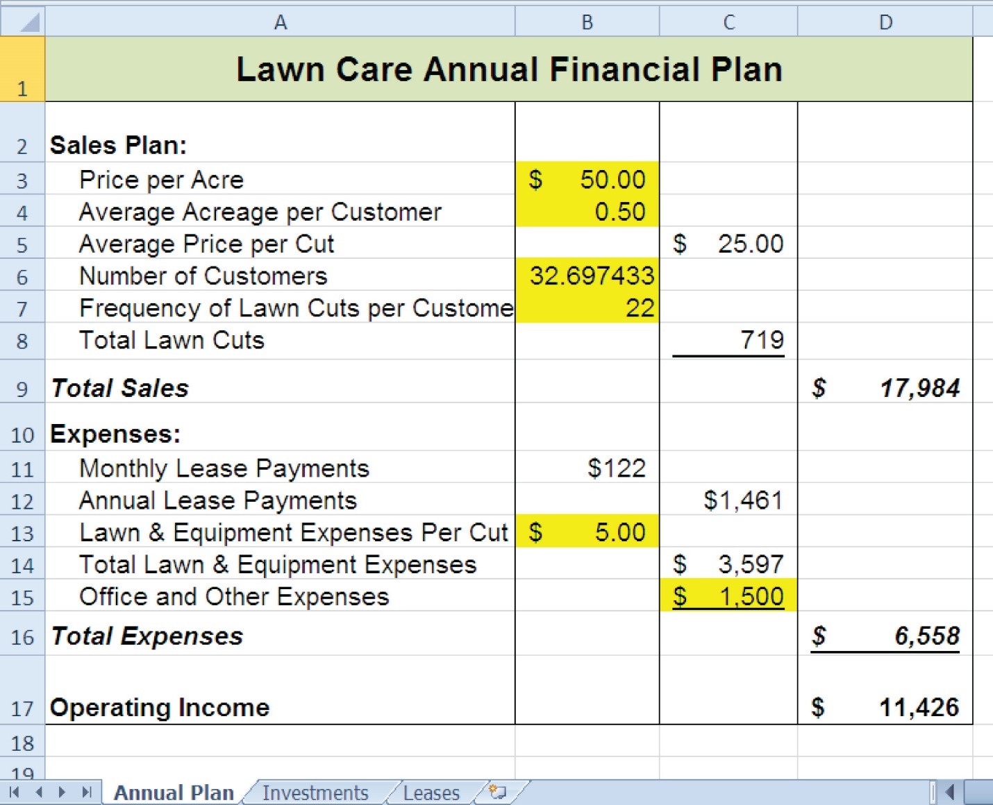
Figure 2.50 Completed CiP Exercise 1 Investments Worksheet
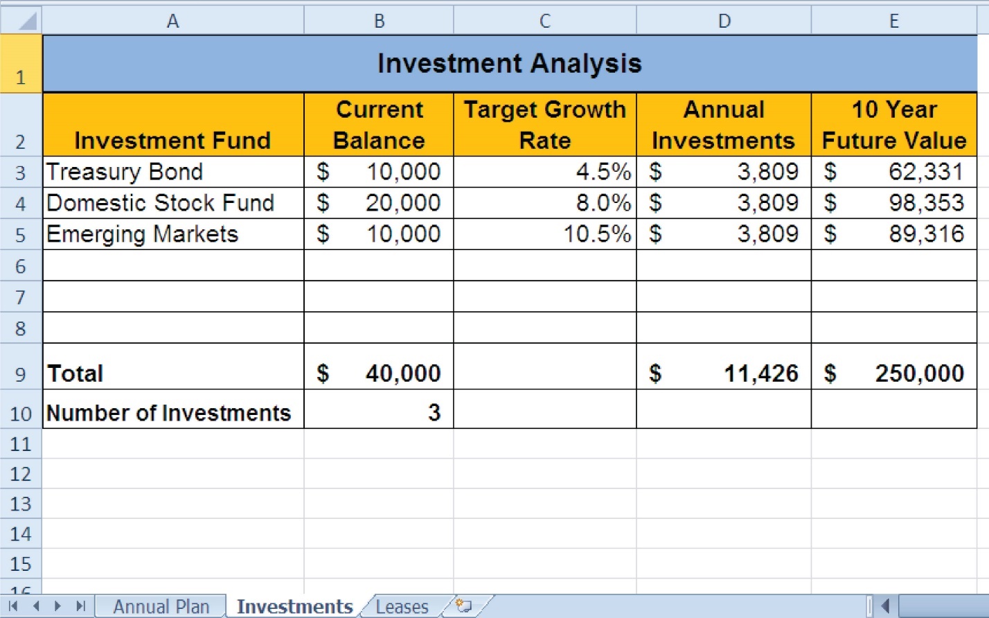
Figure 2.51 Completed CiP Exercise 1 Leases Worksheet