7 Functions for Personal Finance
Functions for Personal Finance
Learning Objectives
- Understand the fundamentals of loans and leases.
- Create and use named cells and ranges in functions.
- Use the PMT function to calculate monthly mortgage payments on a house.
- Use the PMT function to calculate monthly lease payments for an automobile.
- Learn how to summarize data in a workbook using worksheet links to create a summary worksheet.
- Understand the concept of the time value of money.
- Use the FV function to calculate the future value of personal investments.
In this section, we will discover the power of using named cells and ranges in our functions to better describe what is happening inside the function itself as we continue to develop the Personal Budget workbook. Notable items that are missing from the Budget Detail worksheet are the payments you might make for a car or a home. In addition, you may want to set and track a savings goal. This section demonstrates Excel functions used to calculate lease payments for a car, to calculate mortgage payments for a house, and to project future savings based on regular contributions and an average rate of return. This section also discusses the scenario capabilities of Excel once the Personal Budget workbook is complete. Before we continue with our Budget worksheet, we will explore how to name cells and ranges, modify them, rename them, or delete them.
Defining and using names in formulas
By using names, you can make your formulas much easier to understand and maintain. You can define a name for a cell, a range of cells, a function, a constant, or a table. Once you adopt the practice of using names in your workbook, you can easily update, audit, and manage these names. A name is a meaningful shorthand that makes it easier to understand the purpose of a cell reference, constant, formula, or table, each of which may be difficult to comprehend at first glance. The following information shows common examples of names and how they can improve clarity and understanding.
| Example Type | Example With No Name | Example Using a Name |
| Reference | =SUM(C20:C30) | =SUM(FirstQuarterSales) |
| Constant | =PRODUCT(A5,8.3) | =PRODUCT(Price,WASalesTax) |
| Formula | =SUM(VLOOKUP(A1,B1:F20,5,FALSE),-G5) | =SUM(VLOOKUP(Inventory_Level,-Order_Amt,FALSE) -G5 |
| Table | C4:G36 | =TopSales06 |
Types of names
There are several types of names that you can create and use.
Defined name – A name that represents a cell, range of cells, formula, or constant value. You can create your own defined name, and Microsoft Office Excel sometimes creates a defined name for you, such as when you set a print area.
Table name – A name for an Excel table, which is a collection of data about a particular subject that is stored in records (rows) and fields (columns). We will discuss Tables later.
The scope of a name – All names have a scope, either to a specific worksheet (also called the local worksheet level) or to the entire workbook (also called the global workbook level). The scope of a name is the location within which the name is recognized without qualification. For example:
• If you have defined a name, such as Budget_FY18, and its scope is Sheet1, that name, if not qualified, is recognized only in Sheet1, but not in other sheets without qualification. To use a local worksheet name in another worksheet, you can qualify it by preceding it with the worksheet name, as the following example shows: Sheet1! Budget_FY18
• If you have defined a name, such as Sales_Dept_Goals, and its scope is the workbook, that name is recognized for all worksheets in that workbook, but not for any other workbook.
A name must always be unique within its scope. You can override the local worksheet level for all worksheets in the workbook, except for the first worksheet, which always uses the local name if there is a name conflict and cannot be overridden.
Defining and entering names
You define a name by using the:
• Name box on the formula bar. This is best used for creating a workbook level name for a selected range.
• Create a name from selection. You can conveniently create names from existing row and column labels by using a selection of cells in the worksheet.
• New Name dialog box. This is best used for when you want more flexibility in creating names, such as specifying a local worksheet level scope or creating a name comment.
Note: By default, names use absolute cell references.
You can select named cells and ranges to use in your functions and formulas by:
• Typing: Typing the name, for example, as an argument to a formula.
• Using Formula AutoComplete: Use the Formula AutoComplete drop-down list, where valid names are automatically listed for you.
• Selecting from the Use in Formula command: Select a defined name from a list in the Use in Formula command in the Defined Names group on the Formulas ribbon.
Pasting a defined names list:
You can also create a list of defined names in a workbook. Locate an area with two empty columns on the worksheet (the list will contain two columns, one for the name and one for a description of the name). Select a cell that will be the upper-left corner of the list. On the Formulas tab, in the Defined Names group, click Use in Formula, click Paste Names and then, in the Paste Names dialog box, click Paste List.
Naming Rules
The following is a list of naming rules that you need to be aware of when you create and edit names.
• Valid characters: The first character of a name must be a letter, an underscore character (_), or a backslash (\). Remaining characters in the name can be letters, numbers, periods, and underscore characters.
Tip: You cannot use the uppercase and lowercase characters “C”, “c”, “R”, or “r” as a defined name, because they are all used as a shorthand for selecting a row or column for the currently selected cell when you enter them in a Name or Go To text box.
• Cell references disallowed – Names cannot be the same as a cell reference, such as Z$100 or R1C1.
• Spaces are not valid: Spaces are not allowed as part of a name. Use the underscore character (_) and period (.) as word separators, such as, Sales_Tax or First.Quarter.
• Name length – A name can contain up to 255 characters.
• Case sensitivity – Names can contain uppercase and lowercase letters. Excel does not distinguish between uppercase and lowercase characters in names. For example, if you created the name Sales and then create another name called SALES in the same workbook, Excel prompts you to choose a unique name.
Define a name for a cell or cell range on a worksheet
1. Select the cell, range of cells, or non adjacent selections that you want to name.

2. Click the Name box at the left end of the formula bar.
3. Type the name that you want to use to refer to your selection. Names can be up to 255 characters in length.
4. Press ENTER.
Note: You cannot name a cell while you are changing the contents of the cell.
Define a name by using a selection of cells in the worksheet
You can convert existing row and column labels to names.
1. Select the range that you want to name, including the row or column labels.
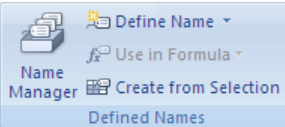
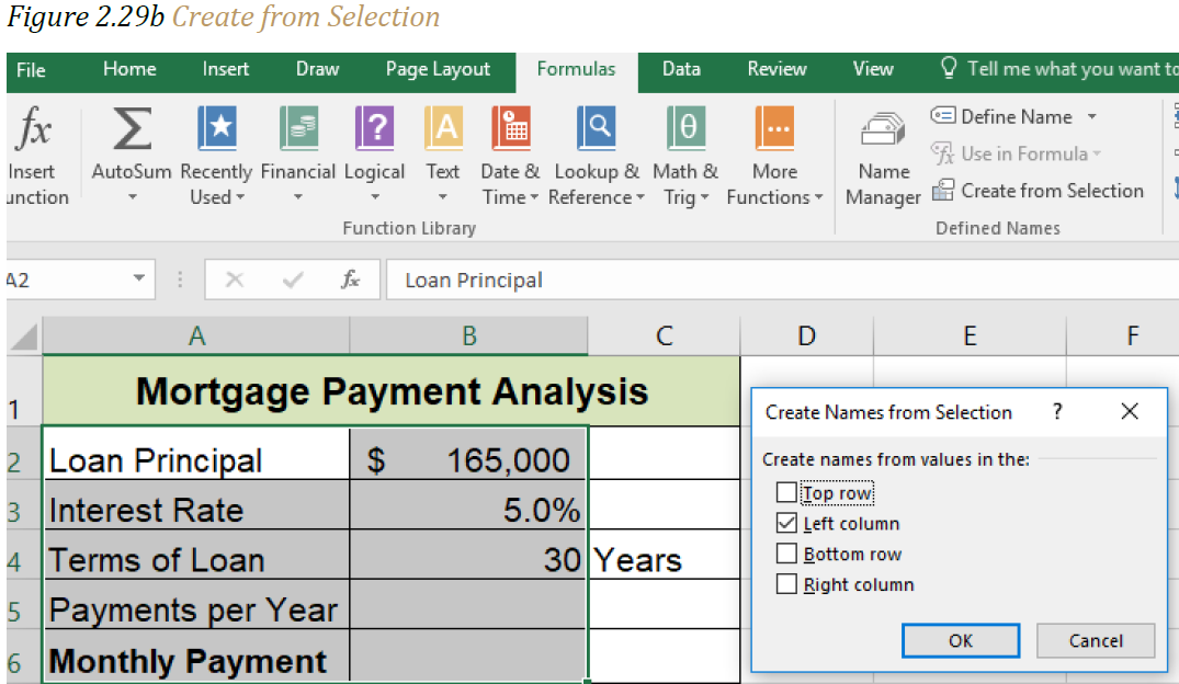
2. On the Formulas tab, in the Defined Names group, click Create from Selection.
In the Create Names from Selection dialog box, designate the location that contains the labels by selecting the Top row, Left column, Bottom row, or Right column check box. A name created by using this procedure refers only to the cells that contain values and does not include the existing row and column labels.
Define a name by using the New Name dialog box
1. On the Formulas tab, in the Defined Names group, click Define Name.
2. In the New Name dialog box, in the Name box, type the name that you want to use for your reference. Note: Names can be up to 255 characters in length.
3. To specify the scope of the name, in the Scope drop-down list box, select Workbook or the name of a worksheet in the workbook.
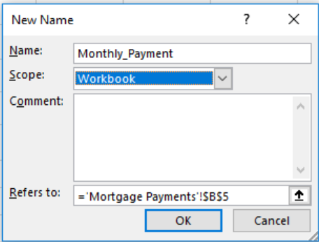
4. Optionally, in the Comment box, enter a descriptive comment up to 255 characters.
5. In the Refers to box, do one of the following:
o To enter a cell reference, type the cell reference.
o If a cell or range of cells has already been selected, you can leave it.
o You can use the up arrow to the right of the” Refers to:” to verify your cell or range reference.
Tip: The current selection is entered by default. To enter other cell references as an argument, click Collapse Dialog (which temporarily shrinks the dialog box), select the cells on the worksheet, and then click Expand Dialog.
o To enter a constant, type = (equal sign) and then type the constant value.
o To enter a formula, type = and then type the formula.
6. To finish and return to the worksheet, click OK.
Tip: To make the New Name dialog box wider or longer, click and drag the grip handle at the bottom.
Manage names by using the Name Manager dialog box
Use the Name Manager dialog box to work with the defined names and table names in the workbook. For example, you may want to find names with errors, confirm the value and reference of a name, view or edit descriptive comments, determine the scope, or delete a named range or cell. You can sort and filter the list of names, and easily add, change, or delete names from one location.
To open the Name Manager dialog box, on the Formulas tab, in the Defined Names group, click Name Manager.
View names
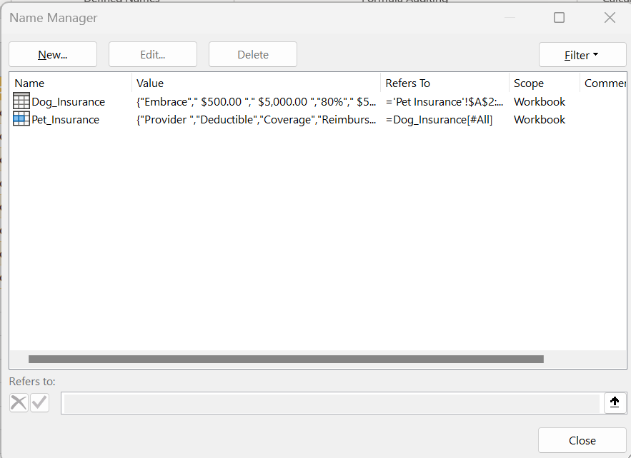
The Name Manager dialog displays the following information about each name in a list box:
Icon and Name One of the following:
• A defined name, which is indicated by a defined name icon.
• A table name, which is indicated by a table name icon.
Value:
The current value of the name, such as the results of a formula, a string constant, a cell range, an error, an array of values, or a placeholder if the formula cannot be evaluated.
Refers To:
The current cell reference or cell reference range for the name.
Scope: One of the following:
• A worksheet name, if the scope is the local worksheet level.
• “Workbook”, if the scope is the global worksheet level.
Comment:
Additional information about the name up to 255 characters.
Note: You cannot use the Name Manager dialog box while you are changing the contents of the cell.
Change a name
If you change a defined name or table name, all uses of that name in the workbook are also changed.
1. On the Formulas tab, in the Defined Names group, click Name Manager.
2. In the Name Manager dialog box, click the name that you want to change, and then click Edit.
Tip: You can also double-click the name.
3. In the Edit Name dialog box, in the Name box, type the new name for the reference.
4. In the Refers to box, change the reference, and then click OK.
5. In the Name Manager dialog box, in the Refers to box, change the cell, formula, or constant represented by the name.
o To cancel unwanted or accidental changes, click Cancel, or press ESC.
o To save changes, click Commit, or press ENTER.
The Close button only closes the Name Manager dialog box. It is not required to commit changes that have already been made.
Delete one or more names
1. On the Formulas tab, in the Defined Names group, click Name Manager.
2. In the Name Manager dialog box, click the name that you want to change.
3. Select one or more names by doing one of the following:
o To select a name, click it.
o To select more than one name in a contiguous group, click and drag the names, or press SHIFT and click the mouse button for each name in the group.
o To select more than one name in a noncontiguous group, press CTRL and click the mouse button for each name in the group.
4. Click Delete. You can also press DELETE.
5. Click OK to confirm the deletion. The Close button only closes the Name Manager dialog box. It is not required to commit changes that have already been made.
The Fundamentals of Loans and Leases
Follow-along file: Continue with Excel Objective 2.00. (Use file Excel Objective 2.10 if starting here.)
One of the functions we will add to the Personal Budget workbook is the PMT function. This function calculates the payments required for a loan or a lease. However, before demonstrating this function, it is important to cover a few fundamental concepts on loans and leases.
A loan is a contractual agreement in which money is borrowed from a lender and paid back over a specific period of time. The amount of money that is borrowed from the lender is called the principal of the loan. The borrower is usually required to pay the principal of the loan plus interest. When you borrow money to buy a house, the loan is referred to as a mortgage. This is because the house being purchased also serves as collateral to ensure payment. In other words, the bank can take possession of your house if you fail to make loan payments. As shown in Table 2.5 “Key Terms for Loans and Leases”, there are several key terms related to loans and leases.
| Term | Definition |
| Residual Value | The estimated selling price of a vehicle at a future point in time. |
| Terms | The amount of time you have to repay a loan. |
| Collateral | Any item of value that is used to secure a loan to ensure payments to the lender. |
| Down Payment | The amount of cash paid toward the purchase of an asset. If you are paying 20% down, you are paying 20% of the cost of the asset in cash and are borrowing the rest from a lender. |
| Interest Rate | The interest that is charged to the borrower as a cost for borrowing money. |
| Mortgage | A loan where property is put up for collateral. |
| Principal | The amount of money borrowed from a lender. |
Figure 2.29 “Example of an Amortization Table” shows an example of an amortization table for a loan. A lender is required by law to provide borrowers with an amortization table when a loan contract is offered. The table in the figure shows how the payments of a loan would work if you borrowed $100,000 from a lender and agreed to pay it back over 10 years at an interest rate of 5%. You will notice that each time you make a payment, you are paying the bank an interest fee plus some of the loan principal. Each year the amount of interest paid to the bank decreases and the amount of money used to pay off the principal increases. This is because the bank is charging you interest on the amount of principal that has not been paid. As you pay off the principal, the interest rate is applied to a lower number, which reduces your interest charges. Finally, the figure shows that the sum of the values in the Interest Payment column is $29,505. This is how much it costs you to borrow this money over 10 years. Indeed, borrowing money is not free. It is important to note that to simplify this example, the payments were calculated on an annual basis. However, most loan payments are made monthly.

A lease is a contract in which you, the lessee, use an asset such as a car or a piece of equipment and you agree to make regular payments to the owner or the lessor. When you lease a car, the manufacturer or a leasing company retains ownership of the vehicle and you agree to make regular payments for a specific period of time. The amount of money you pay depends on the price of the car, the terms of the lease contract, and the car’s expected residual value at the end of the lease. The calculation of lease payments is like the calculation of loan payments. However, when you lease a car, you pay only the value of the car that is used. For example, suppose you are leasing a car that is priced at $25,000. The lease contract is for 4 years at an interest rate of 5%. The residual value of the car is $10,000. This means the car will lose $15,000 of its value over 4 years. Another way to state this is that the car will depreciate $15,000. A lease will be structured so that you pay this $15,000 in depreciation. However, the interest charges will be based on the purchase price of $25,000. We will look at a demonstration of leasing a car as well as buying a home in the next section.
The PMT (Payment) Function for Loans
Follow-along file: Continue with Excel Objective 2.00. (Use file Excel Objective 2.10 if starting here.)
If you own a home, your mortgage payments are a major component of your household budget. If you are planning to buy a home, having a clear understanding of your monthly payments is critical for maintaining strong financial health. In Excel, mortgage payments are conveniently calculated through the PMT (payment) function. This function is more complex than the statistical functions covered in Section 2.2 “Statistical Functions”. With statistical functions, you are required to add only a range of cells or selected cells within the parentheses of the function. With the PMT function, you must accurately define a series of arguments for the function to produce a reliable output. Table 2.6 “Arguments for the PMT Function” lists the arguments for the PMT function. It is helpful to review the key loan and lease terms in Table 2.5 “Key Terms for Loans and Leases” before reviewing the PMT function arguments.
The PMT function is: =PMT (RATE,NPER,PV,[FV],[Type])
| Argument | Definition |
| Rate | This is the interest rate the lender is charging the borrower. The interest rate is usually quoted in annual terms, so you must divide this rate by the number of payments per year. |
| Nper | The argument letters stand for number of periods. This is the term of the loan, which is the amount of time you have to repay the bank. This is usually quoted in years, so you must multiply the years by numbers of payments per year. |
| Pv | The argument letters stand for present value. This is the principal of the loan or the amount of money that is borrowed. When defining this argument, a minus sign must precede the cell location or value. For leases. this argument is used for the price of the item being leased. |
| [Fv] | The argument letters stand for future value. The brackets around the argument indicate that it is not always necessary to define it. It is used if there is a lump-sum payment that will be made at the end of the loan terms. This is also used for the residual value of a lease. If it is not defined, Excel will assume that it is zero. |
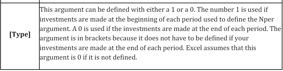
| Type | This argument can be defined with either a 1 or a 0. The number 1 is used if payments are made at the beginning of each period. A 0 is used if payments are made at the end of each period. The argument is in brackets because it does not have to be defined if payments are made at the end of each period. Excel assumes that this argument is 0 if it is not defined. |
We will use the PMT function in the Personal Budget workbook to calculate the monthly mortgage payments for a house. These calculations will be made in the Mortgage Payments worksheet and then displayed in the Budget Summary worksheet through a named cell reference link.
The first thing we will do in this worksheet is name the cells we will be using in our functions. Next, we will discover a new method of adding functions to a worksheet. The following steps explain the new method using the Insert Function command for adding the PMT function:
1. Click the Mortgage Payments worksheet tab.
2. Highlight the range A2:B6. On the Formula ribbon, Defined Names section click on Create from Selection. Make sure Left Column is checked. (see Figure 2.29b “Create from Selection”). Click OK. You have now named all of the cells in the B column. (You can verify your named cells by using the drop-down arrow in the Name Box.)
3. Click cell B5.
4. Click the Formulas tab on the Ribbon.
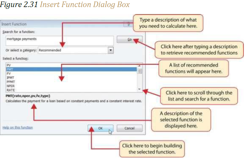
5. Click the Insert Function button (see Figure 2.30 “Mortgage Payments Worksheet”). This opens the Insert Function dialog box, which can be used for searching all functions in Excel.
6. In the “Search for a function:” input box at the top of the Insert Function dialog box, type payment (see Figure 2.31 “Insert Function Dialog Box”). Note that the current description in the “Search for a function:” input box will already be highlighted. You can begin typing and the description will be replaced with your entry.
7. Click the Go button in the upper right side of the Insert Function dialog box. This adds all the Excel functions that match your description in the “Select a function:” box in the lower half of the Insert Function dialog box (see Figure 2.31 “Insert Function Dialog Box”).
8. Click the PMT option in the “Select a function:” box in the lower half of the Insert Function dialog box.
9. Click the OK button at the lower right side of the Insert Function dialog box. This will open the Function Arguments dialog box.

Keyboard Shortcuts – Insert Function
Hold the SHIFT key while pressing the F3 key.
10. The cursor automatically starts in the Rate box. This will be the first argument defined for the PMT function.
11. Click cell B3 on the worksheet. This is the rate being charged on the loan. You will see your defined name Interest_Rate appear in the Rate argument box.
12. Type a forward slash (/) for division.
13. Click on cell B5. Since our goal is to calculate the monthly payments for the loan, we need to divide the rate, which is stated in annual terms, by the number of payments per year. The number of payments per year is found in cell B5. This converts the annual rate to a monthly rate. (periodic rate) Your defined name Payments_per_Year will appear after your /.
14. Click in the Nper field in the Function Arguments dialog box. This is the second argument we define in the function. Nper is the total number of payments to be made over the life of the loan. It is the loan in years * the payments per year.
15. Click cell B4 on the worksheet. This is the term or the amount of time we have to repay the loan. You will see the defined name Terms_of_Loan appear in your Nper argument box.
16. Type an asterisk (*) for multiplication.
17. Click on cell B5. Since our goal is to calculate the total number of payments for the loan, we need to multiply the term of the loan by payments per year.
18. Click in the Pv argument field in the Function Arguments dialog box. This is the third argument we will define in the function.
19. Type a minus sign (−). When defining the Pv argument of the PMT function, any cell location or value must be preceded with a minus sign.
20. Click cell B2 on the worksheet. This is the principal of the loan. Your defined name Loan_Principal will appear in the PV argument field.
21. You will now see the Rate, Nper, and Pv arguments defined for the function.
22. Click the OK button at the bottom of the Function Arguments dialog box. The function will now be placed into the worksheet. Since we are not paying any lump sums of money at the end of the loan, there is no need to define the Fv argument. Also, we will assume that the monthly mortgage payments will be made at the end of each month. Therefore, there is no need to define the Type argument.
Figure 2.32 “Function Arguments Dialog Box for the PMT Function” shows the completed Function Arguments dialog box for the PMT function. Notice that the dialog box shows the values for the Rate and Nper arguments. The Rate is divided by 12 to convert the annual interest rate to a monthly interest rate. The Nper argument is multiplied by 12 to convert the terms of the loan from years to months. Finally, the dialog box provides you with a definition for each argument. The definition appears when you click in the input box for the argument.
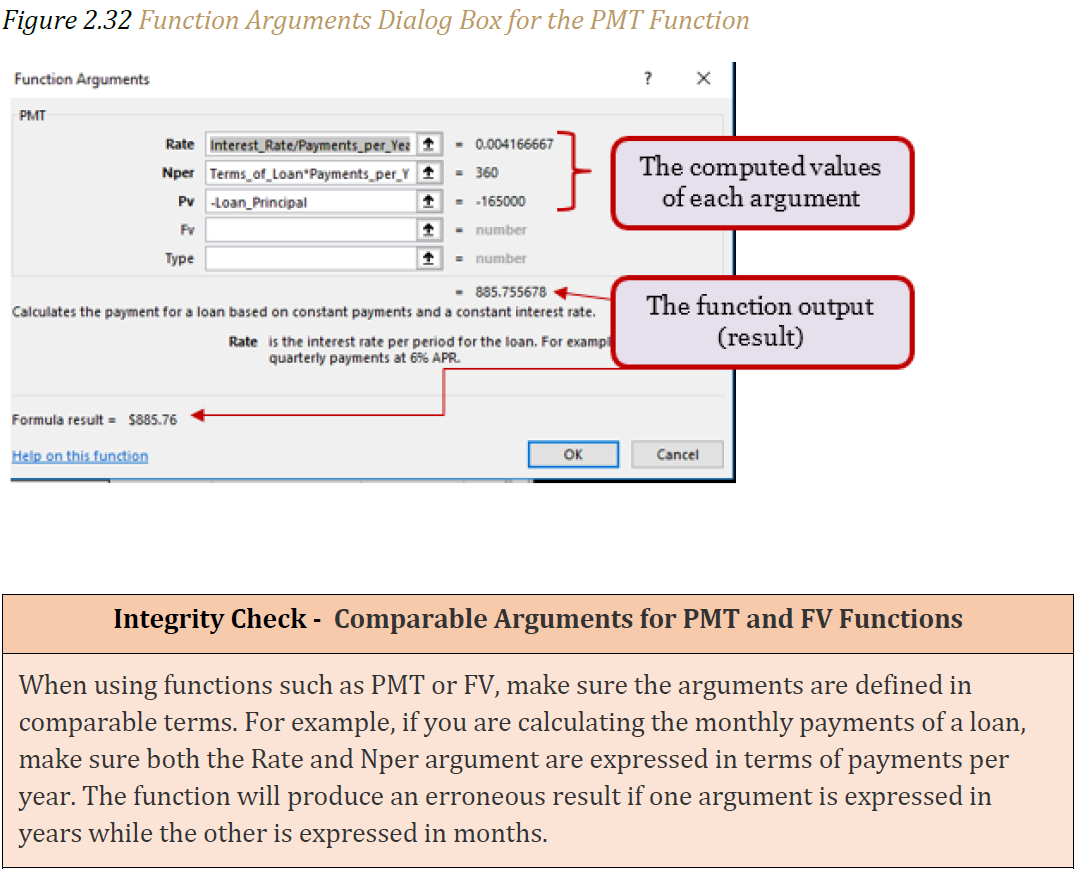
Figure 2.33 “Mortgage Payments Worksheet with the PMT Function” shows the final appearance of the Mortgage Payments worksheet after the PMT function is added. The result of the function in cell B6 will be displayed in the Budget Summary worksheet.

The PMT (Payment) Function for Leases
Follow-along file: Continue with Excel Objective 2.00. (Use file Excel Objective 2.11 if starting here.)
In addition to calculating the mortgage payments for a home, the PMT function will be used in the Personal Budget workbook to calculate the lease payments for a car. The details for the lease payments are found in the Car Lease Payments worksheet. Similar to the statistical functions, we can type the PMT function directly into a cell. However, you must know the definitions for each argument of the function and understand how these arguments need to be defined based on your objective. The terms for loans and leases are in Table 2.5 “Key Terms for Loans and Leases”, and the definitions for the arguments of the PMT function are in Table 2.6 “Arguments for the PMT Function”. The following steps explain how the PMT function is added to the Personal Budget workbook to calculate lease payments for a car:
1. Highlight the range A2:B6. On the Formula ribbon, Defined Names section click on Create from Selection. Make sure Left Column is checked. (see Figure 2.29b “Create from Selection”). Click OK. You have now named all of the cells in the B column. (You can verify you named cells by using the drop-down arrow in the Name Box.)
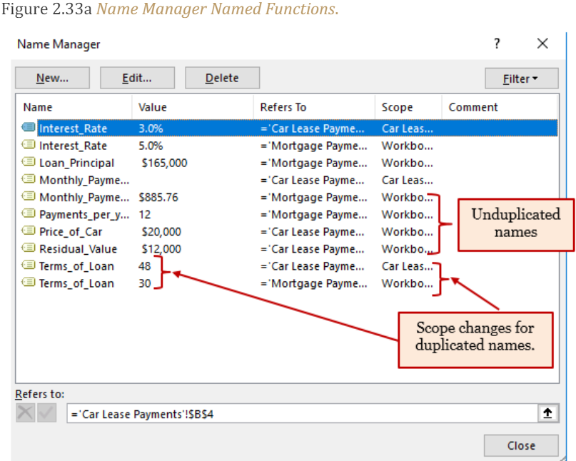
Note: When we use the same names on two different worksheets, the Name Manager assigns a different scope. The first time we named Interest rate the scope was for the Mortgage Payments worksheet. This time it is for the Car Lease Payments worksheet. See Figure 2.33a.
2. Click cell B6 in the Car Lease Payments worksheet.
3. Type an equal sign (=).
4. Type the letters PMT. A drop-down list of Excel functions will appear. Double click PMT.

5. Click cell B4. This is the interest rate being charged for the lease.
6. Type the forward slash (/) for division.
7. Type the number 12. Since our goal is to calculate the monthly lease payments, we divide the interest rate by 12 to convert the annual rate to a monthly rate.
8. Type a comma. When you type a function containing arguments, you must separate each argument with a comma. This signals to Excel that one argument has been defined and you are ready to define the next argument in the function.
9. Click cell B5. This is the term or the length of time for the lease contract. Since the term is already expressed in months, we can just reference cell B5 and move to the next argument.
10. Type a comma. This advances the function to the Pv argument.
11. Type a minus sign (−). Remember that cell locations or values used to define the Pv argument must be preceded with a minus sign.
12. Click cell B2 on the worksheet, which is the price of the car.
13. Type a comma. This advances the function to the [Fv] argument.
14. Click cell B3 on the worksheet. This is the residual value of the car. Note that cell location and values used to define the [Fv] argument are NOT preceded by a minus sign.
15. Type a comma. This advances the function to the [Type] argument.
16. Type the number 1. We will assume that the lease payments will be due at the beginning of each month.
17. Type a closing parenthesis ()).
18. Press the ENTER key.
19. Figure 2.34 “PMT Function Constructed to Calculate Lease Payments” shows how the PMT function should appear before pressing the ENTER key. Notice the commas that separate each argument of the function. Also, the tip box will show the current argument being defined in bold font.
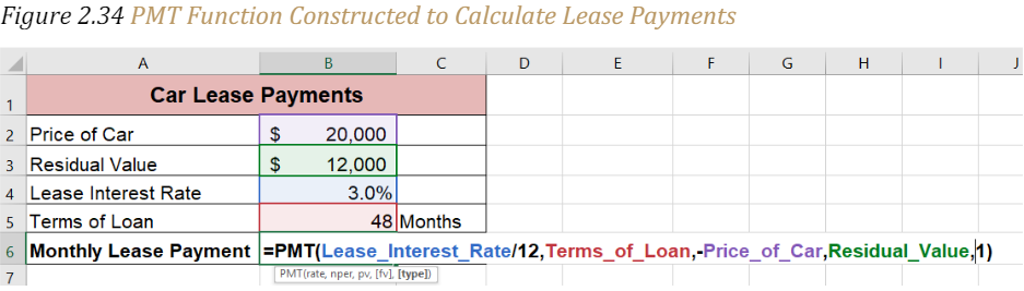
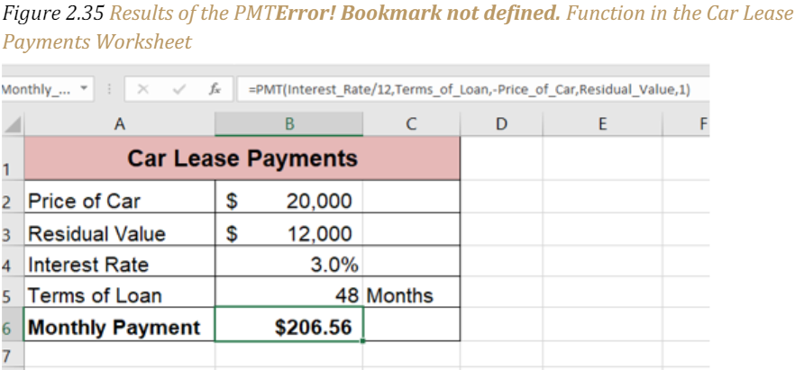
Figure 2.35 “Results of the PMT Function in the Car Lease Payments Worksheet” shows the result of the PMT function. The monthly payments for this lease are $206.56. This monthly payment will be displayed in the Budget Summary worksheet.
Figure 2.35 Results of the PMT Function in the Car Lease Payments Worksheet
Creating an Amortization Schedule for a Loan
Follow-along file: Continue with Excel Objective 2.00. (Use file Excel Objective 2.11b if starting here.)
Now that we have determined how much a loan or lease will cost per month, it is useful to determine how interest and principal will be applied from our payment each month. Figure 2.35b shows how interest and principal on a loan behave over time. You can see from this chart that it will take you over 16 years for your payments to go more toward principal than interest.
One of the advantages of preparing an amortization schedule is that you can see exactly how much is being applied to principal and interest each time you make a payment. You can also play with the monthly payment amount and see how increasing your payment will apply more to your principal payment while reducing your loan duration.

To complete the amortization schedule, we will use two financial functions; the PPMT Principal Payment function that calculates the amount of any given period’s principal payment, and the IPMT Interest Payment function, which calculates the interest taken from any given period payment. The PPMT and the IPMT have the same arguments and are the same as the PMT with one exception. The exception is that you must tell the function which period you are calculating out the interest or principal.
The arguments in either function are:
RATE, Current period, NPER, PV
• Where RATE = the periodic interest rate (RATE/payments per year)
• Current period = the current period number
• NPER = total payments over the life of the loan
• PV = the original amount of the loan
Let’s set up an amortization schedule. Complete the following steps:
1. On the Mortgage Payments worksheet enter the following column headers:
a. Cell A9: Payment Number
b. Cell B9: Beginning Balance
c. Cell C9: Principal Payment
d. Cell D9: Interest Payment
e. Cell E9: Ending Balance
2. Highlight cells B9:C9 and Wrap Text. Increase columns to letters in words stay together.
3. Highlight cells A9:E9 and apply an All Borders style from the Font section of the Home ribbon.
4. In cell A10 enter the number 1
5. In cell A11 enter the number 2
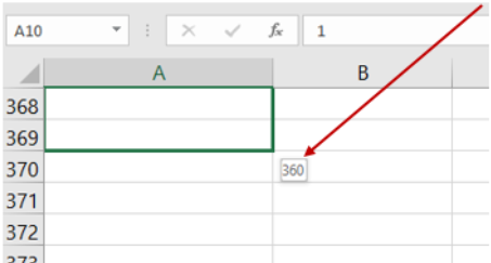
6. Highlight cells A10:A11 and use the Fill handle at the bottom right corner of A11 to drag down until you have 360 payments in column A. Note: The Fill handle will show you what number you have filled through outside the lower right corner.
7. In cell B10 enter = and click on the Loan principal in cell B2.
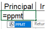
8. In cell C10 enter the PPMT function =PPMT, then double click on the function in the box below the cell.
9. To complete the function
a. Click on cell B3 (Interest Rate) enter the / to divide the rate, click on B5 (Payment per year).
b. Enter a comma to separate the arguments.
c. Click on cell A10 to enter the current period, enter a comma,
d. Click on cell B4 to enter the Term of the loan, enter an * to multiply the term by the payments per year in cell B5
e. Enter a – minus sign and then click on B2 for the Loan Principal amount.
f. Close your PPMT function with a closing ). The figure below shows the arguments after they have been entered into the function. (The cells were already named in this worksheet.)-

10. In cell D10 inter the IPMT function using the steps for the PPMT above, except you will type the IPMT instead of PPMT.
11. In cell E10 subtract the principal payment in cell C10 from the beginning balance in cell B10. =B10-C10
12. In cell B11 enter = and click on the ending balance in cell E10.
13. Highlight the range C10:E10 and copy down one row. (Using the fill handle makes this easy.)
14. Highlight the cells B11:E11 and use the fill handle to fill the formulas down through the 360th payment. You can do this quickly by double clicking the fill handle in the lower right corner of your highlighted area border. The balance in the last cell should = 0.
Linking Worksheets with 3-D Cell References. (Creating a Summary Worksheet)
Follow-along file: Continue with Excel Objective 2.00. (Use file Excel Objective 2.12 if starting here.)
So far, we have used cell references and named cells in formulas and functions, which allows Excel to produce new outputs when the values in the cell references are changed. Cell references can also be used to display values or the outputs of formulas and functions in cell locations on other worksheets. This is how data will be displayed on the Budget Summary worksheet in the Personal Budget workbook. Outputs from the formulas and functions that were entered into the Budget Detail, Mortgage Payments, and Car Lease Payments worksheets will be displayed on the Budget Summary worksheet using 3-D cell references. The following steps explain how this is accomplished:
1. Click cell C3 in the Budget Summary worksheet.
2. Type an equal sign (=).
3. Click the Budget Detail worksheet tab.
4. Click cell D12 on the Budget Detail worksheet.
5. Press the ENTER key on your keyboard. The output of the SUM function in cell D12 on the Budget Detail worksheet will be displayed in cell C3 on the Budget Summary worksheet.
Figure 2.36 “Cell Reference Showing the Total Expenses in the Budget Summary Worksheet” shows how the cell reference appears in the Budget Summary worksheet. Notice that the cell reference D12 is preceded by the Budget Detail worksheet name enclosed in apostrophes followed by an exclamation point (‘Budget Detail’!) This indicates that the value displayed in the cell is referencing a cell location in the Budget Detail worksheet.
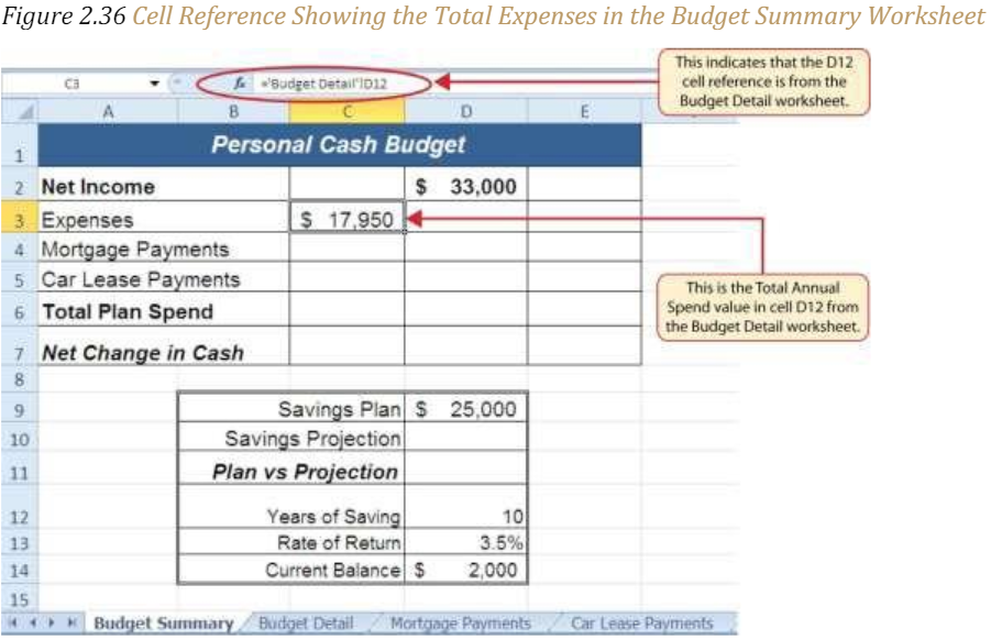
As shown in Figure 2.36 “Cell Reference Showing the Total Expenses in the Budget Summary Worksheet”, the Budget Summary worksheet is designed to show the expense budget for the mortgage payments and the auto lease payments. However, you will recall that we used the PMT function to calculate the monthly payments. In the Budget Summary worksheet, we need to show the total annual payments. As a result, we will create a formula that references cell locations in the Mortgage Payments and Car Lease Payments worksheets. The following steps explain how this is accomplished:
1. Click cell C4 in the Budget Summary worksheet.
2. Type an equal sign (=).
3. Click the Mortgage Payments worksheet tab.
4. Click cell B5 in the Mortgage Payments worksheet.
5. Type an asterisk (*) for multiplication.
6. Type the number 12. This multiplies the monthly payments by 12 to calculate the total payments required for the year.
7. Press the ENTER key on your keyboard. The value of multiplying the monthly mortgage payments by 12 is now displayed on the Budget Summary worksheet.
8. Click cell C5 on the Budget Summary worksheet.
9. Type an equal sign (=).
10. Click the Car Lease Payments worksheet tab.
11. Click cell B6 in the Car Lease Payments worksheet.
12. Type an asterisk (*) for multiplication.
13. Type the number 12. This multiplies the monthly lease payments by 12 to calculate the total payments required for the year.
14. Press the ENTER key on your keyboard. The value of multiplying the monthly lease payments by 12 is now displayed on the Budget Summary worksheet.
15. Highlight cells C4:C5, format Comma with no decimal places.
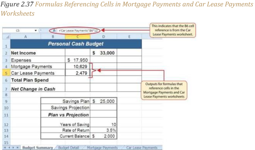
Figure 2.37 “Formulas Referencing Cells in Mortgage Payments and Car Lease Payments Worksheets” shows the results of creating formulas that reference cell locations in the Mortgage Payments and Car Lease Payments worksheets.
We can now add other formulas and functions to the Budget Summary worksheet that can calculate the difference between the total spend dollars vs. the total net income in cell D2. The following steps explain how this is accomplished:
1. Click cell D6 in the Budget Summary worksheet.
2. Click on AutoSum at in the Editing section of the Home ribbon
3. Highlight the range C3:C5
4. Click Enter.
5. Click cell D7 on the Budget Summary worksheet.
6. Type an equal sign (=).
7. Click cell D2.
8. Type a minus sign (−) and then click cell D6.
9. Press the ENTER key on your keyboard. This formula produces an output of $1,942, indicating our income is greater than our total expenses.
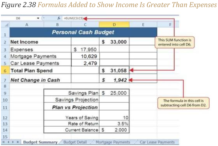
Figure 2.38 “Formulas Added to Show Income Is Greater Than Expenses” shows the results of the formulas that were added to the Budget Summary worksheet. The output for the formula in cell D7 shows that the net income exceeds total planned expenses by $1,942. Overall, having your income exceed your total expenses is a good thing because it allows you to save money for future spending needs or unexpected events.
We can now add a few formulas that calculate both the spending rate and the savings rate as a percentage of net income. These formulas require the use of absolute references, which we covered earlier in this chapter. The following steps explain how to add these formulas:
1. Click cell E6 in the Budget Summary worksheet.
2. Type an equal sign (=).
3. Click cell D6.
4. Type a forward slash (/) for division and then click D2.
5. Press the F4 key on your keyboard. This adds an absolute reference to cell D2.
6. Press the ENTER key. The result of the formula shows that total expenses consume 94.1% of our net income.
7. Click cell E6.
8. Place the mouse pointer over the Autofill Handle.
9. When the mouse pointer turns to a black plus sign, left click and drag down to cell E7. This copies and pastes the formula into cell E7.
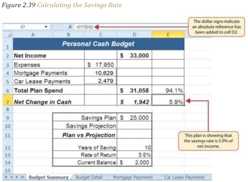
Figure 2.39 “Calculating the Savings Rate” shows the output of the formulas calculating the spending rate and savings rate as a percentage of net income. The absolute reference shown for cell D2 prevents the cell from changing when the formula is copied from cell E6 and pasted into cell E7. The results of the formula show that our current budget allows for a savings rate of 5.9%. This is a fairly good savings rate. In the next section, we will discuss how these savings can grow over time by exploring the time value of money concepts.
Time Value of Money Concepts
Follow-along file: Continue with Excel Objective 2.00. (Use file Excel Objective 2.13 if starting here.)
In reviewing the Budget Summary worksheet in Figure 2.39 “Calculating the Savings Rate”, you will notice that the range B9:D14 contains data that can be used to assess a savings plan. We can project how much money can be saved over a specific period of time given set contributions and a rate of return. This calculation is accomplished through the future value, or FV, function. We will use the FV function in cell D10 of the Budget Summary worksheet to calculate our savings plan projection. However, before we use the FV function, it is important to review a few basic concepts regarding the time value of money, as shown in Table 2.7 “Key Terms for Time Value of Money Concepts”.
Table 2.7 “Key Terms for Time Value of Money Concepts” provides definitions for several terms used when addressing the time value of money concepts. The time value of money is the opportunity to grow your money over time given a constant or average rate of return.
| Argument | Definition |
| Annuity | An investment that is made in regular payments over a period of time. For example, depositing $100 a month into an interest-bearing bank account or mutual fund is considered an annuity. |
| Bonds | An investment in which you lend money to a company or government entity. The borrower agrees to pay you interest over a specific period of time. At the end of the bond agreement, the amount of money that was borrowed, or your initial investment, is returned to you. Most bonds are considered a lower risk investment but offer a lower rate of return than stocks offer. |
| Mutual Funds | A collection of similar investments managed by a financial professional called a fund manager. Mutual funds allow you to invest in several stocks or bonds without having to make any individual investments. They also allow you to reduce your risk and take advantage of the investment expertise of a professional. |
| Rate of Return | The percentage gained or lost on an investment. Investments that offer a high predicted rate of return often carry a higher risk of losing money. Investments that offer a lower predicted rate of return often carry a lower risk of losing money. |
| Stocks | An investment in which a purchaser owns a portion of a company. The value of this investment increases as the company produces higher profits. Most stocks are expected to produce a higher rate of return than bonds generate. However, the risk of losing money on a stock investment is much greater than the risk for bonds. |
For example, consider the data shown in Figure 2.40 “Time Value of Money Example for a One-Time Investment”. This data assumes that a person makes a one-time investment of $100 in a bond mutual fund that returns 5% interest per year. Notice that the interest paid in Column E increases every year. This is because the interest is reinvested in the mutual fund, which increases the total value of the investment. For example, the interest earned in year 1 is based on a $100 investment. Therefore, the interest paid is $5.00, or 5% of $100. However, in year 2, when the $5.00 interest payment is reinvested, the total investment increases to $105. Therefore, in year 2 the interest paid increases to $5.25, or 5% of $105. The value of the investment at the end of 5 years is $127.63. This is the value that can be calculated using the FV function.
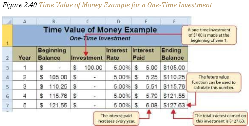
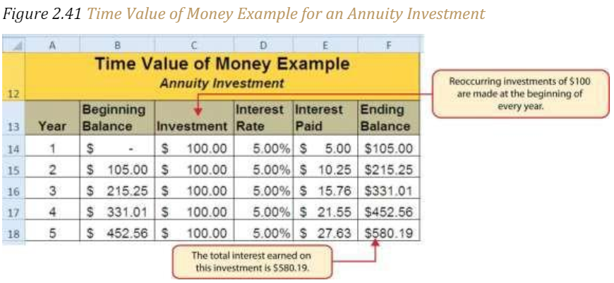
Figure 2.41 “Time Value of Money Example for an Annuity Investment” shows another example demonstrating the time value of money concept. Instead of making a one-time investment, we will assume that a person invests $100 at the beginning of every year in the same bond mutual fund. This is referred to as an annuity because the person is making reoccurring investments over a specific period of time. Notice that the value of this investment after 5 years is $580.19. Also, the total interest earned on this investment is $80.19 as opposed to the $27.63 earned on the one-time investment in Figure 2.40 “Time Value of Money Example for a One-Time Investment”.
The FV (Future Value) Function
Follow-along file: Continue with Excel Objective 2.00. (Use file Excel Objective 2.13 if starting here.)
Establishing a personal savings plan is one of the most important financial exercises you can do. For example, a savings plan is critical for establishing financial security for your retirement years. Many people mistakenly believe that saving for retirement is something you do when you get older. However, the greatest financial gains for your retirement can be achieved if you start saving in the earliest years of your career. Now that you understand the time value of money, you can see that the more years you can earn interest on your investments and reinvest those earnings, the more money you will have when you retire. Savings plans are also important for other key life events, such as going to college or buying a home.
FV = (RATE, NPER, PMT,[PV],[TYPE])
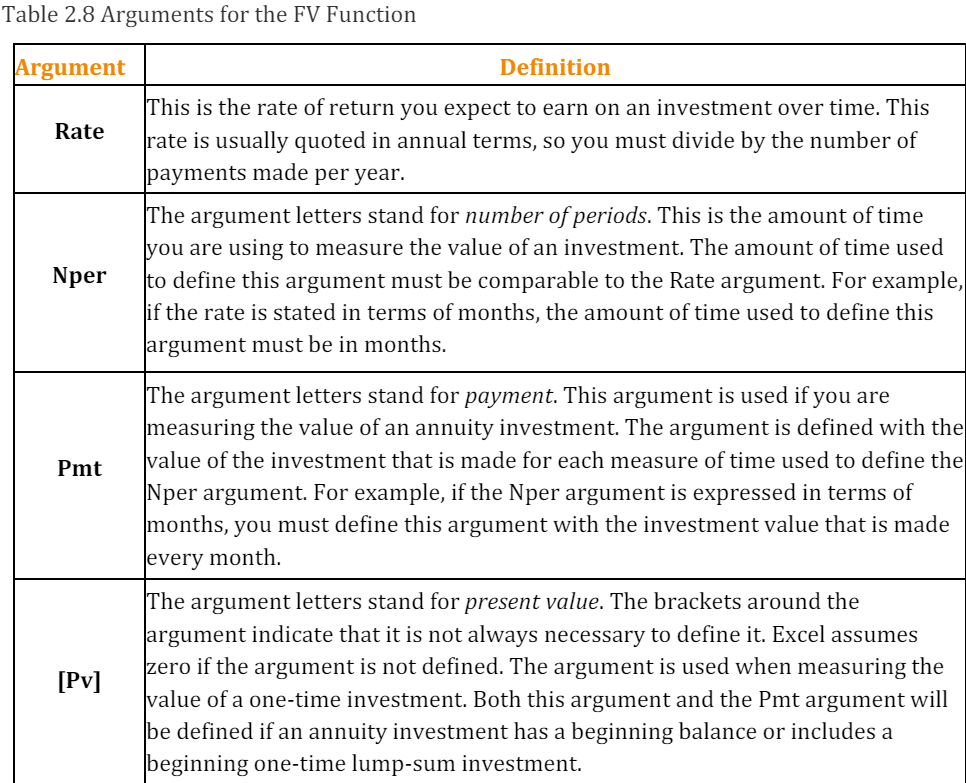
The FV function is a convenient tool that can help you establish savings goals and project the value of your investments over time. Like the PMT function, the FV function requires you to accurately define specific arguments in order to produce a reliable result. Table 2.8 “Arguments for the FV Function” provides definitions for each of the arguments in the FV function. It is helpful to review the time value of money terms in Table 2.7 “Key Terms for Time Value of Money Concepts” before using the FV function.
With respect to the Personal Budget workbook, we will use the FV function to project the value of the savings plan in 10 years. We will type the function directly into the Personal Budget worksheet for this demonstration. However, you can use any of the methods demonstrated in this chapter for future use.
The following steps explain how this function is added to the worksheet:
- Click cell D10 in the Budget Summary worksheet.
- Type an equal sign (=).
- Type the letters FV followed by an open parenthesis (().
- Click cell D13. This is the expected rate of return for the investments.
- Type a comma.
- Click cell D12. This is the amount of time the investments are expected to grow.
- Type a comma.
- Type a minus sign (−). All values or cell locations used to define the PMT argument must be preceded by a minus sign.
- Click cell D7. This is the change in cash that was calculated by subtracting the total expenses from the net income. We are expecting to save this amount of money for the 10-year period this investment is being measured.
- Type a comma.
- Type a minus sign (−). All values and cell locations used to define the Pv argument must be preceded by a minus sign.
- Click cell D14. Since the savings plan has a current balance, we use this to define the Pv argument of the function. This is equivalent to starting with a lump-sum investment.
- Type a closing parenthesis ()). There is no need to define the last argument of the function because we will assume that the savings in cash achieved in our budget will be invested at the end of each year of the savings plan. Press the ENTER key Now we will check to see if our savings plan is over, or short of, its goal.
- Check that cell D11 is activated.
- Type an equal sign (=).
- Click cell D10.
- Type a minus sign (−) and then click cell D9. This subtracts the savings plan from the current savings plan projection.
- Press the ENTER key.
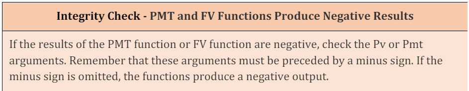
Figure 2.42 “Results of the Savings Plan Projections” shows the results of the FV function. Notice that the current savings plan projection is $25,606. This is $606 higher than the target of $25,000 entered into cell D9, which shows that the current budget is working to achieve the goals of this savings plan. In other words, given the current net income, we are saving enough money to achieve our savings plan goals.
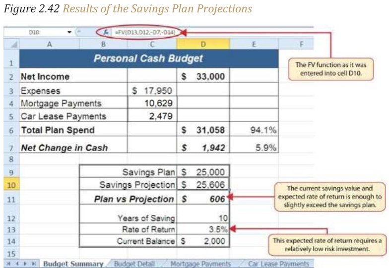
There are two important factors to notice about this plan. The first factor is that our spending plan allows us to save enough money so that it can be invested to achieve our target of $25,000. The second factor is that the expected rate of return is 3.5%. This is a relatively low expected rate of return and could be achieved by investing in relatively lowrisk investments such as bonds as opposed to stocks. This rate can be considered good because we can achieve our savings goals without having to make high-risk investments that could result in a significant loss of our savings. If the results of the PMT function or FV function are negative, check the Pv or Pmt arguments. Remember that these arguments must be preceded by a minus sign. If the minus sign is omitted, the funct.ions produce a negative output.
NPER
Follow-along file: Continue with Excel Objective 2.00. (Use file Excel Objective 2.14 if starting here.)
Given the home loan example above there are other financial functions that can be used to help make financial decisions when borrowing money. For instance, if we can afford to pay $1,000 per month for our loan and the bank will loan to us at 5% interest on a $165,000 loan, how long will it take to pay off that loan?
The NPER function solves for the total number of payments it will take to pay off this loan. The function is:
=NPER (RATE,PMT,-PV,[FV],[Type])
Return to the Mortgage Payments worksheet and complete the following steps:
1. In cell E1 type: What if Analysis
2. In cell E2 type: Years to payoff loan if: (NPER)
3. In cell E4 type: Payment per month:
4. In cell E5 enter $1,000
5. In G2 enter =NPER (
6. Click on cell B3 – the interest rate in the mortgage analysis section. Enter the divisor (/) and click on the Payments per year in cell B5 to calculate the periodic interest rate. Type a comma.
7. Click on the $1,000 in cell F3 for the PMT argument and then enter a comma.
8. Enter a minus sign (-) and click on B2, the Loan Principal and then hit Enter. The result shows 279.74 payments.
9. To solve for the number of years we must divide the total number of payments by the payments per year. Click in the formula bar for G3. After the closing parenthesis divide (/) the result by the payments per year in cell B5.
10. Format cell G3 for comma with one decimal place.
Figure 2.43 shows the result that being able to pay an extra $115 per month on a 30-year loan will cut 7 years off the length of this loan.

RATE
Follow-along file: Continue with Excel Objective 2.00. (Use file Excel Objective 2.15 if starting here.)
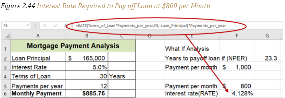
Another what if analysis you can play with when making financial decisions around loans is what is the highest interest rate you can afford to pay given your financial situation. Let’s assume that the most we can afford to pay monthly for the loan is $800. Everything else will remain the same in our Mortgage analysis, but we will know before entering into a loan how much interest we can afford. We will do this by solving for the RATE.
The RATE function solves for the periodic interest rate. The arguments in the function are:
=RATE (NPER,PMT, -PV,[FV],[Type])
1. On the Mortgage Payments worksheet, in cell E5 type: Payment per month.
2. In F5, type: $800
3. In cell E6, type Interest rate (RATE)
4. In cell F6 enter =RATE (
5. Calculate the NPER by clicking on cell B4 and multiply (*) by B5. Enter a comma
6. Enter the payment amount by clicking on cell F5 and enter a comma
7. Enter a minus sign (-) and click on the loan principal in cell B2.
8. Finish the function by typing the closing parenthesis.
9. The result in cell F6 may show 0%. Increase decimal places to show 3 decimal places. The periodic interest rate is 0.344%. To calculate the annual interest rate, you must multiply the result of the RATE function by the number of payments per year.
10. Make cell F6 active and click in the formula bar. At the end of your RATE function multiply the function by payments per year in B5.
Figure 2.44 shows the results of the RATE function. You would have to get an interest rate of 4.125% to be able to afford the $165,000 house at $800 per month.