3 Formatting and Data Analysis

Formatting and Data Analysis

This section addresses formatting commands that can be used to enhance the visual appearance of a worksheet. It also introduces mathematical calculations and charts. The skills introduced in this section will give you powerful tools for analyzing the data that we have been working with in this workbook and will highlight how Excel is used to make key decisions in virtually any career.

Formatting Data and Cells

Follow-along file: Excel Objective 1.0 (Use file Excel Objective 1.04 if starting with this skill.)

Enhancing the visual appearance of a worksheet is a critical step in creating a valuable tool for you or your coworkers when making key decisions. The following steps demonstrate several fundamental formatting skills that will be applied to the workbook that we are developing for this chapter. Several of these formatting skills are identical to ones that you may have already used in other Microsoft applications such as Microsoft® Word® or Microsoft® PowerPoint®.

1. Highlight the range A2:D2 in the Sheet1 worksheet by placing the mouse pointer over cell A2 and left clicking and dragging to cell D2.

2. Click the Bold button in the Font group of commands in the Home tab of the Ribbon (see Figure 1.36 “Font Group of Commands”).

Figure 1.36 Font Group of Commands

3. Highlight the range B15:D15 by placing the mouse pointer over cell A15 and left clicking and dragging to cell D15.

4. Click the Bold button in the Font group of commands in the Home tab of the Ribbon.

5. Click the Italics button in the Font group of commands in the Home tab of the Ribbon.

6. Highlight the range B15:D15. Click the drop-down arrow next to the Borders button in the Font group of commands in the Home tab of the Ribbon. From the drop-down, select the Top and Double Bottom border style. This is a standard business/accounting presentation of totals in a worksheet and denotes the end of a set of data.

Figure 1.36b Border Icon

7. Highlight the range B3:B14 by placing the mouse pointer over cell B3 and left clicking and dragging down to cell B14.

8. Click the Comma Style button in the Number group of commands in the Home tab of the Ribbon.

Figure 1.37 Number Group of Commands

9. Click the Decrease Decimal button in the Number group of commands in the Home tab of the Ribbon (see Figure 1.37 “Number Group of Commands”).

10. The numbers will also be reduced to zero decimal places.

11. Highlight the range C3:D3 by placing the mouse pointer over cell C3 and left clicking and dragging across to cell D3.

12. Click the Accounting Number Format button in the Number group of commands in the Home tab of the Ribbon (see Figure 1.37 “Number Group of Commands”). This will add the US currency symbol and two decimal places to the values. This format is common when working with pricing data.

13. Highlight the range C4:D14 by placing the mouse pointer over cell D3 and left clicking and dragging down to cell D14.

14. Click the Comma symbol to the values as well as two decimal places.

15. Highlight D3:D14 and click the Decrease Decimal button twice in the Number group of commands in the Home tab of the Ribbon. You are decreasing the decimals to none because the Sales Dollars do not have any cents displayed. Decimal places when only zeroes are displayed adds clutter to your worksheet.

16. This will add the comma style to the values and reduce the decimal places to zero. The comma style aligns the numbers in the cells with the Accounting style where $ are displayed.

17. Highlight the range A1:D1 by placing the mouse pointer over cell A1 and left clicking and dragging over to cell D1.

18. Click the down arrow next to the Fill Color button in the Font group of commands in the Home tab of the Ribbon (see Figure 1.38 “Fill Color Palette”).

19. Click the Aqua, Accent 5, Darker 25% color from the palette (see Figure 1.38 “Fill Color Palette”). Notice that as you move the mouse pointer over the color palette, you will see a preview of how the color will appear in the highlighted cells.

Figure 1.38 Fill Color Palette

20. Click the down arrow next to the Font Color button in the Font group of commands in the Home tab of the Ribbon (see Figure 1.36 “Font Group of Commands”), and select White for the font color. This change will be visible once text is typed into the highlighted cells.

21. Click the Increase Font Size button in the Font group of commands in the Home tab of the Ribbon (see Figure 1.38 “Fill Color Palette”). Each click will increase the font size 1 point.

22. Highlight the range A1:D15 by placing the mouse pointer over cell A1 and left clicking and dragging down to cell D15.

23. Click the drop-down arrow on the right side of the Font button in the Home tab of the Ribbon (see Figure 1.36 “Font Group of Commands”).

24. Notice that as you move the mouse pointer over the font style options, you can see the font change in the highlighted cells.

25. Expand the row width of Column D to 10 characters.

Figure 1.39 “Formatting Techniques Applied” shows how the Sheet1 worksheet should appear after the formatting techniques are applied.

Figure 1.39 Formatting Techniques Applied

1.4 Data Alignment

Data Alignment (Wrap Text, Merge Cells, and Center)

Follow-along file: Excel Objective 1.0 (Use file Excel Objective 1.06 if starting with this skill.)

The skills presented in this segment show how data are aligned within cell locations. For example, text and numbers can be centered in a cell location, left justified, right justified, and so on. In some cases, you may want to stack multiword text entries vertically in a cell.

instead of expanding the width of a column. This is referred to as wrapping text. These skills are demonstrated in the following steps:

1. Highlight the range B2:D2 by placing the mouse pointer over cell B2 and left clicking and dragging over to cell D2.

2. Click the Center button in the Alignment group of commands in the Home tab of the Ribbon (see Figure 1.40 “Alignment Group in Home Tab”). This will center the column headings in each cell location.

Figure 1.40 Alignment Group in Home Tab

3. Click the Wrap Text button in the Alignment group (see Figure 1.40 “Alignment Group in Home Tab”). The height of Row 2 automatically expands, and the words that were cut off because the columns were too narrow are now stacked vertically (see Figure 1.42 “Sheet1 with Data Alignment Features Added”).

4. Highlight the range A1:D1 by placing the mouse pointer over cell A1 and left clicking and dragging over to cell D1.

5. Click the down arrow on the right side of the Merge & Center button in the Alignment group of commands in the Home tab of the Ribbon.

6. Left click the Merge & Center option (see Figure 1.41 “Merge Cell Drop-Down Menu”). This will create one large cell location running across the top of the dataset with centered text.

Figure 1.41 Merge Cell Drop-Down Menu

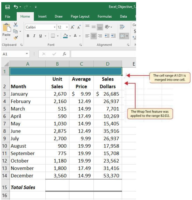
Figure 1.42 “Sheet1 with Data Alignment Features Added” shows the Sheet1 worksheet with the data alignment commands applied. The reason for merging the cells in the range A1:D1 will become apparent in the next segment.

Figure 1.42 Sheet1 with Data Alignment Features Added

Creating Multi-Line Worksheet Titles

Your worksheets need to tell their story without a person there to explain them. They need to be clearly labeled and formatted for ease of understanding. However, one important part of the story that often gets left out is the title of the story. All worksheets should include an

informative title that describes the contents of the worksheet and the date, or range of dates, the data pertains to. We will include a title.

Follow-along file: Excel Objective 1.0 (Use file Excel Objective 1.07 if starting with this skill.)

In the Sheet1 worksheet, the cells in the range A1:D1 were merged for the purposes of adding a title to the worksheet. This title will require that three lines of text be entered into a cell. The following steps explain how you can enter text into a cell and determine where you want the second line of text to begin:

1. Activate cell A1 in the Sheet1 worksheet by placing the mouse pointer over cell A1 and clicking the left mouse button. Since the cells were merged, clicking cell A1 will automatically activate the range A1:D1.

2. Type the text General Merchandise World.

3. Hold down the ALT key and press the ENTER key. This will start a new line of text in this cell location.

4. Type the text 2017 Retail Sales (in millions) and press the ENTER key.

5. Select cell A1. Then click the Italics button in the Font group of commands in the Home tab of the Ribbon.

6. Increase the height of Row 1 to 30 points. Once the row height is increased, all the text typed into the cell will be visible (see Figure 1.43 “Title Added to the Sheet1 Worksheet”).

Figure 1.43 Title Added to the Sheet1 Worksheet

Borders (Adding Lines to a Worksheet)

Follow-along file: Excel Objective 1.0 (Use file Excel Objective 1.08 if starting with this skill.)

In Excel, adding custom lines to a worksheet is known as adding borders. Borders are different from the grid lines that appear on a worksheet and that define the perimeter of the cell locations. The Borders command lets you add a variety of line styles to a worksheet that can make reading the worksheet much easier.

The following steps illustrate methods for adding preset borders and custom borders to a worksheet:

1. Highlight cells A2:D2.

2. Click the down arrow to the right of the Borders button in the Font group of commands in the Home page of the Ribbon (see Figure 1.44 “Borders Drop-Down Menu”).

Figure 1.44 Borders Drop-Down Menu

3. Left click the All Borders option from the Borders drop-down menu (see Figure 1.44 “Borders Drop- Down Menu”). This will add vertical and horizontal lines to the range A2:D2.

4. Highlight the range A2:D2 by placing the mouse pointer over cell A2 and left clicking and dragging over to cell D2.

5. Click the down arrow to the right of the Borders button.

6. Left click the Thick Bottom Border option from the Borders drop-down menu.

7. Highlight the range A1:D15.

8. Click the down arrow to the right of the Borders button.

9. This will open the Format Cells dialog box (see Figure 1.45 “Borders Tab of the Format Cells Dialog Box”). You can access all formatting commands in Excel through this dialog box.

10. In the Style section of the Borders tab, left click the thickest line style (see Figure 1.45 “Borders Tab of the Format Cells Dialog Box”).

11. Left click the Outline button in the Presets section (see Figure 1.45 “Borders Tab of the Format Cells Dialog Box”).

12. Click the OK button at the bottom of the dialog box (see Figure 1.45 “Borders Tab of the Format Cells Dialog Box”).

Figure 1.45 Borders Tab of the Format Cells Dialog Box

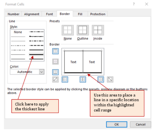
Figure 1.46 Borders Added to the Sheet1 Worksheet

AutoSum

Follow-along file: Excel Objective 1.0 (Use file Excel Objective 1.09 if starting with this skill.)

You will see at the bottom of Figure 1.46 “Borders Added to the Sheet1 Worksheet” that Row 15 is intended to show the totals for the data in this worksheet. Applying mathematical computations to a range of cells is accomplished through functions in Excel. Chapter 2 “Mathematical Computations” will review mathematical formulas and functions in detail. However, the following steps will demonstrate how you can quickly sum the values in a column of data using the AutoSum command:

1. Activate cell B15 in the Sheet1worksheet.

2. From the right side of the Home Ribbon, or the left side of the Formula ribbon, click the down arrow next to the AutoSum button. You will see that the AutoSum can sum, average, count numbers, and create Max and Min functions.

Figure 1.47 AutoSum Drop-Down List

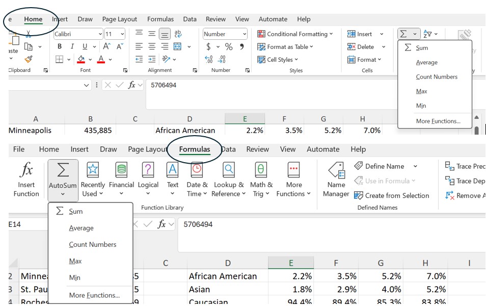
3. The default command for AutoSum is Sum. Select Sum from the drop-down list. (see Figure 1.47 “AutoSum Drop-Down List”). Note that the AutoSum button can also be found in the Editing group of commands in the Home tab of the Ribbon.

4. Excel will provide a total for the values in the Unit Sales column.

5. Click in cell D15 and click the AutoSum button. You will see that with this sum the Accounting format ($) has been applied to your total row. Excel will copy the formatting from your top row as the default number format for your total row. (Note: you should not add the Average Price column because it is only a list of prices.)

Figure 1.48 Totals Added to the Sheet1 Worksheet

1.5 Simple Chart

Inserting a Column Chart

Follow-along file: Excel Objective 1.0 (Use file Excel Objective 1.10 if starting with this skill.)

As mentioned at the beginning of this chapter, Excel serves as a critical tool for making decisions in both personal and professional contexts. Charts are a powerful tool in Excel that allow you to graphically display the data in a worksheet. Graphical displays allow the reader to immediately identify key trends and behaviors in the data that is being analyzed. For the workbook that we are using for this chapter, understanding the trends in monthly sales data is critical for making decisions such as how many staff members to assign to the store for each month as well as supplying the store with enough inventory to accommodate expected sales. To assist the reader in analyzing this data, a column chart will be created to graphically display the data. It is important for you to plan which type of chart will best display the data so your readers can quickly see key trends. More details on creating charts and on chart types will be presented in a later chapter. The following steps are an introduction to creating the column chart required for this chapter’s objective:

1. Highlight the range A2:B14.

2. Click the Insert tab of the Ribbon.

3. Click the Column button (see Figure 1.49 “Column Chart Drop-Down Menu”). This will open the column chart drop-down menu of options.

4. Select the Clustered Column option from the list of column chart options (see Figure 1.49 “Column Chart Drop-Down Menu”). This will create an embedded chart in the Sheet1 worksheet (see Figure 1.50 “Embedded Column Chart in Sheet1”). Embedded means that the chart is on the worksheet that contains the original chart data. The chart is floating on the top of the worksheet and can be moved and sized on the face of the worksheet.

Figure 1.49 Column Chart Drop-Down Menu

Figure 1.50 “Embedded Column Chart in Sheet1” shows the column chart that is created once a selection is made from the column chart drop-down menu. Notice that there are two new tabs added to the Ribbon. These tabs contain features for enhancing the appearance and construction of Excel charts. These commands will be covered in more detail in a later chapter. For now, you will see that Excel places the chart over the data in the worksheet. The following steps explain how to move and resize the chart:.

Figure 1.50 Embedded Column Chart in Sheet1

5. While the chart is selected (buttons are visible around the outside of the chart), left click anywhere it the chart and drag the chart so the upper left corner is placed in the middle of cell F1.

6. Place the mouse pointer over the top center sizing handle (see Figure 1.50 “Embedded Column Chart in Sheet1”). You will see the mouse pointer change from a white block plus sign to a vertical double arrow. Make sure the mouse pointer is not in the cross-arrow mode as this will move the chart instead of resizing it.

7. While holding down the ALT key on your keyboard, left click and drag the mouse pointer slightly up. The chart will automatically adjust up to the top of Row 1.

8. Place the mouse pointer over the left center sizing handle.

9. While holding down the ALT key on your keyboard, left click and drag the mouse slightly toward the left. The chart will automatically adjust to the left side of Column F.

10. Place the mouse pointer over the lower center sizing handle.

11. While holding down the ALT key on your keyboard, left click and drag the mouse slightly down. The chart will automatically adjust to the bottom of Row14.

12. Place the mouse pointer over the right center sizing handle.

13. While holding down the ALT key on your keyboard, left click and drag the mouse slightly to the right. The chart will automatically adjust to the right side of Column M.

Figure 1.52 “Embedded Chart Moved and Resized” shows the column chart moved and resized. Notice that the sizing handles are not visible around the perimeter of the chart. This is because the chart is not activated. Once you click anywhere on the worksheet outside the chart area, the chart is automatically deactivated.

Figure 1.52 Embedded Chart Moved and Resized

As shown in Figure 1.50 “Embedded Column Chart in Sheet1”, when a chart is created, two tabs are added to the Ribbon. The following steps explain how to use a few of the formatting and design features in these tabs:

1. Check to make sure the column chart in Sheet1 is activated. To activate the chart, left click anywhere on the chart.

2. Click the Design tab under the Chart Tools set of tabs on the Ribbon.

3. Click the down arrow on the right side of the Chart Styles section (see Figure 1.53 “Chart Styles in the Design Tab”).

Figure 1.53 Chart Styles in the Design Tab

4. Click Style 9 in the Chart Styles section. This style has a black background with blue columns (see Figure 1.53 “Chart Styles in the Design Tab”).

5. Click the Format tab under the Chart Tools set of tabs on the Ribbon.

6. Click the down arrow on the right side of the WordArt Styles section (see Figure in).

Figure 1.54 WordArt Styles in the Format Tab

7. Click the Blue, Accent 1, Inner Shadow option Notice that as you move the mouse pointer over the WordArt Styles options, the format of the chart title as well as the X and Y axis titles changes.

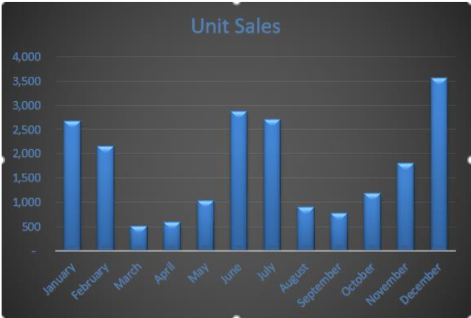
Figure 1.55 “Formatting Features Applied to the Column Chart” shows the embedded column chart with the formatting features applied. This chart is very effective in displaying the Unit Sales trends for this company. You can see very quickly that the tallest bar in the chart is the month of December, followed by the months of June, July, January, and February.

Figure 1.55 Formatting Features Applied to the Column Chart

Cut, Copy, and Paste

Follow-along file: Excel Objective 1.0 (Use file Excel Objective 1.11 if starting with this skill.)

The Cut, Copy, and Paste commands are perhaps the most widely used commands in Microsoft Office. With regard to Excel, the Copy and Paste commands are often used to make copies of worksheets for developing different scenarios or versions for the data being analyzed. The following steps demonstrate how these commands are used for the objective in this chapter:

1. Click the Select All button in the upper left corner of the Sheet1 worksheet (see Figure 1.56 “Clipboard Group of Commands”).

Figure 1.56 Clipboard Group of Commands

2. Click the Copy button in the Clipboard group of commands in the Home tab of the Ribbon (see Figure 1.56 “Clipboard Group of Commands”).

3. Create a new worksheet by clicking on the + button to the right of the Sheet1 tab.

4. Activate cell location A1.

5. Click the Paste button in the Clipboard group of commands in the Home tab of the Ribbon. Be sure to click the upper area of the Paste button and not the down arrow at the bottom of the button. A copy of Sheet1 will now appear in Sheet2.

6. Click anywhere on the chart in the Sheet2 worksheet.

7. Click the Cut button in the Clipboard group on the Home tab of the Ribbon. This will remove the chart from the Sheet2 worksheet.

8. Open the Sheet3 worksheet by left clicking on the Sheet3 worksheet tab at the bottom of the workbook.

9. Activate cell location A1.

10. Click the Paste button in the Home tab of the Ribbon. This will paste the chart from the Sheet2 worksheet into the Sheet3worksheet.

Sorting Data (One Level)

Follow-along file: Excel Objective 1.0 (Use file Excel Objective 1.12 if starting with this skill.)

As mentioned earlier in this section, a chart is a tool that enables worksheet readers to analyze data quickly to spot key trends or patterns. Another powerful tool that provides similar benefits is the Sort command. This feature ranks the rows of data in a worksheet based on designated criteria. The following steps demonstrate how the Sort command is used to rank the data in the Sheet2 worksheet:

1. In the Sheet2 worksheet, highlight the range A2:D14

2. Click the Data tab of the Ribbon.

3. Click the Sort button in the Sort & Filter group of commands. This will open the Sort dialog box (see Figure 1.57 “Sort & Filter Group of Commands”).

Figure 1.57 Sort & Filter Group of Commands

4. Click the down arrow next to the “Sort by” drop-down box in the Sort dialog box (see Figure 1.58 “Sort Dialog Box”). Make sure the box “My data has headers” is checked.

Figure 1.58 Sort Dialog Box

5. Click the Unit Sales option from the drop-down list.

6. Click the down arrow next to the Order drop-down list.

7. Click Largest to Smallest from the drop-down list.

8. Click the OK button at the bottom of the Sort dialog box. The data in the range A2:D14 will now be sorted in descending order based on the values in the Unit Sales column.

(Note that when you perform the sort, your chart will automatically change to match the new sorted data.)

Figure 1.59 “Data Sorted Based on Unit Sales” shows the data in the Sheet2 worksheet sorted based on the values in the Unit Sales column. Similar to the chart, the Sort command makes it easy to identify the months of the year with the highest unit sales.

Figure 1.59 Data Sorted Based on Unit Sales

Moving, Renaming, Inserting, and Deleting Worksheets

Follow-along file: Excel Objective 1.0 (Use file Excel Objective 1.13 if starting with this skill.)

The default names for the worksheet tabs at the bottom of workbook are Sheet1, Sheet2, and so on. However, you can change the worksheet tab names to identify the data you are using in a workbook. Additionally, you can change the order in which the worksheet tabs appear in the workbook. The following steps explain how to rename and move the worksheets in a workbook:

1. With the left mouse button, double click the Sheet1 worksheet tab at the bottom of the workbook (see Figure 1.60 “Renaming a Worksheet Tab”).
2. Type the name Sales by Month.
3. Press the ENTER key on your keyboard.
4. With the left mouse button, double click the Sheet2 worksheet tab at the bottom of the workbook.
5. Type the name Unit Sales Rank.
6. Press the ENTER key on your keyboard.
   

   

    

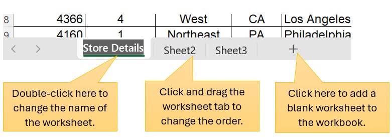
7. Left click and drag the Unit Sales Rank worksheet tab to the left of the Sales by Month worksheet tab.
8. Right click the Sheet3 worksheet tab. Click Delete to delete the worksheet. Alternatively, you can:

1. 1. Click the Home tab of the Ribbon.
   2. Click the down arrow on the Delete button in the Cells group of commands.
   3. Click the Delete Sheet option from the drop-down list (see Figure 1.35 “Delete Drop-Down Menu”).
   4. Click the Delete button on the Delete warning box.

9. Click the Insert Worksheet tab at the bottom of the workbook (see Figure 1.60 “Renaming a Worksheet Tab”).

Figure 1.61 “Final Appearance of the Excel Objective 1.0 Workbook” shows the final appearance of the Excel Objective 1.0 workbook after the worksheet tabs have been renamed and moved.