19 Filtering Data
Filtering Data
Learning Objectives
- Duplicate worksheets.
- Apply number and text filters to a data range.
- Clear Filters
Suni now wants to determine which vehicles should be considered for replacement. She is going to base her decision to replace a vehicle based on the age of the vehicle and the odometer reading. She wants you to filter so that only the vehicles that were purchased before 2008 and have an odometer reading greater than 100,000 miles are shown in the list.
Apply Filters
You could accomplish Suni’s task by copying the worksheet and deleting all the rows of vehicles that don’t meet her criteria, or you can filter the list to only show those vehicles that meet the given criteria. We will use filters to accomplish our goal.
When you create an Excel table, or turn on the Filter from the Data tab, the filter arrows appear next to the column headers. You can use the options on the AutoFilter to create three types of filters. You can filter a column of data by its cell colors or font colors, by a specific text, number or date filter, (although the choices depend upon the type of data in the column,) or by selecting the exact values by which you want to filter in the column. After you filter a column, the Clear Filter command becomes available so you can remove the filter and redisplay all the records.
Follow-along file: Continue with Excel Objective 5.00. (Use file Excel Objective 5.05 if starting here.)
We will set up the filter for Suni, but we want to maintain the first worksheet sort. We will accomplish this by duplicating our worksheet and performing the filter on the new worksheet.
1. While holding the Ctrl key down, left click the worksheet tab and drag to the right. You will see a little image of a piece of paper with a +. Drop the worksheet to the right of the original worksheet. The new worksheet will have the name College Vehicles (2).
2. Rename the worksheet Vehicle Filter.

3. Make sure the Vehicle Filter worksheet is active by clicking on the worksheet tab at the bottom of the worksheet.
4. We will filter on the year first. It doesn’t matter which category you decide to filter on first, the end results will be the same. Click the Category Filter arrow next to Year.

5. The AutoFilter menu opens as shown in Figure 5.7. It lists all the unique entries in the category. The list will differ based upon which column you select to filter.
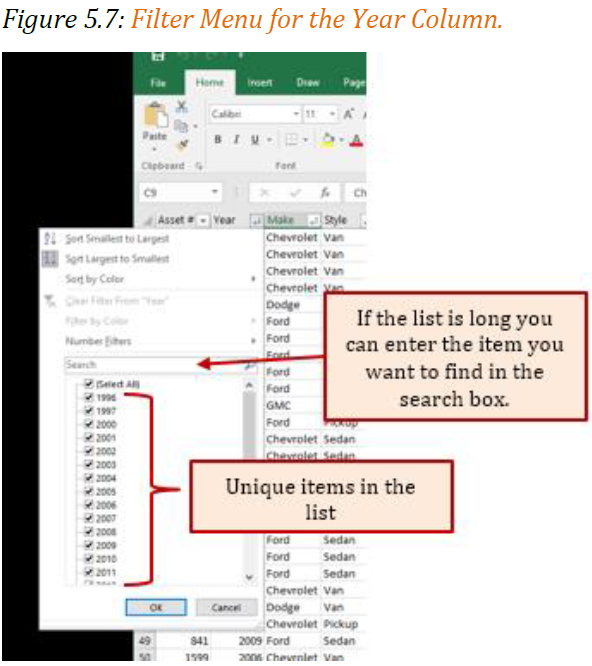
6. We could go through and uncheck all the years we don’t want to filter on. In this case vehicle newer than 2008, or we can use the number filter feature. Click on the Number Filter directly above the Search box. Because we are filtering on all cars older than 2008, we will Select Less Than from the drop-down menu.

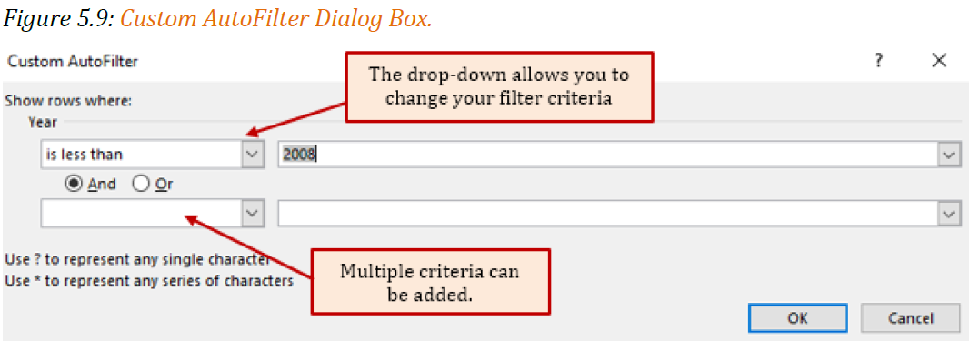
7. In the Custom AutoFilter dialog box, type 2008 and click OK.
8. The next filter we will apply will be for the odometer reading greater than 100,000 miles. Click on the Category Filter arrow next to Odometer and choose Number Filters, Greater than. Type 100000 (no commas) into the criteria value box. Click OK. Figure 5.10 shows the results of the number filters applied to the Year and Odometer columns.
Suni decides that only the Maintenance department will get new vehicles this round, so she wants you to only show Maintenance in your report.
9. Click on the Category Filter next in the Department column. Note that the selection only shows those departments that are included in the filters that have been applied so far. Click the Select All so it is unchecked and then check Maintenance.
10. Click OK to save the filter.
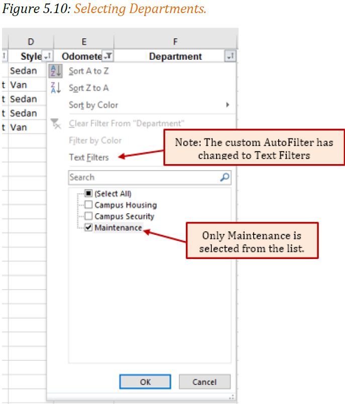
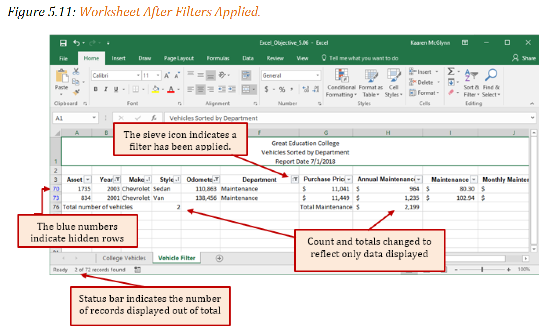
Figure 5.11 shows the results of the custom filters applied to the data. Note that the count of vehicles and the sum of the annual maintenance has changed to reflect only those vehicles included in the filter.
11. The title of the worksheet must be corrected to reflect the data filters applied. We will change the second row of the title to reflect this change. Click in the A1, the worksheet title. Use the down arrow at the right side of the formula bar to show the entire title.
12. Click in the second row and delete the text currently there. Replace that text with Maintenance Dept. Vehicles Bought before 2008 with > 100,000 miles.

Clearing Filters
To redisplay all the data in a filtered table or data range, you need to clear or remove the filters. When you clear a filter from a column, all the other filters still applied will remain in place. To redisplay the entire data table, all the filters must be removed. You can remove filters one at a time, or clear all filters.
To remove one at a time, click on the AutoFilter button next to the category you want to restore. From the drop-down select Clear Filter from…
To remove all filters, click on Clear Filters from the Sort & Filter section of the Data tab.
Key Takeaways
When you are working with a range of data or an Excel table that contains hundreds of thousands of records, filters help you find information quickly and efficiently without having to look at each individual record. For example, you could narrow the search to one student out of a student population of 40,000.
Filtering limits the data to display only the specific records that meet the criterial you set, enabling you to more effectively analyze the data. The following examples further illustrate how filtering can narrow the data to only that data needed.
- Looking for customers in a specific zip code, or range of zip codes.
- Finding those records that have been highlighted by a specific color.
- Searching by customers who purchased from you before a certain date so you can target them for a marketing campaign.
