17 Creating an Excel Table

Creating an Excel Table

Creating a Table

Suni works in the accounting department for Great Education College. She is given the task of condensing the data around vehicles owned by the college. She must condense the information into easily understandable reports to be provided to the college board’s finance committee.

Follow-along file: Excel Objective 5.00.

Suni examines the data in the College Vehicles worksheet. She notes that each has an Asset number, the year vehicle was made, the make and style of the vehicle, which department has control of the vehicle, its purchase price and estimated annual maintenance cost. She will use this data to create her various reports.

A few things to know about data in tables before we begin.

• Data must be in contiguous cells – no breaks in rows or columns

• Headers must be next to the first row of data – no break in rows between headers and the start of your data.

We will create an Excel table to manipulate her data. The steps we will use to do that are:

1. Click on any cell within the list of data.

2. From the Insert ribbon, select Table. Excel will automatically determine the absolute range of cells that will be placed in your table. See Figure 5.01 Excel’s Selection of Data.

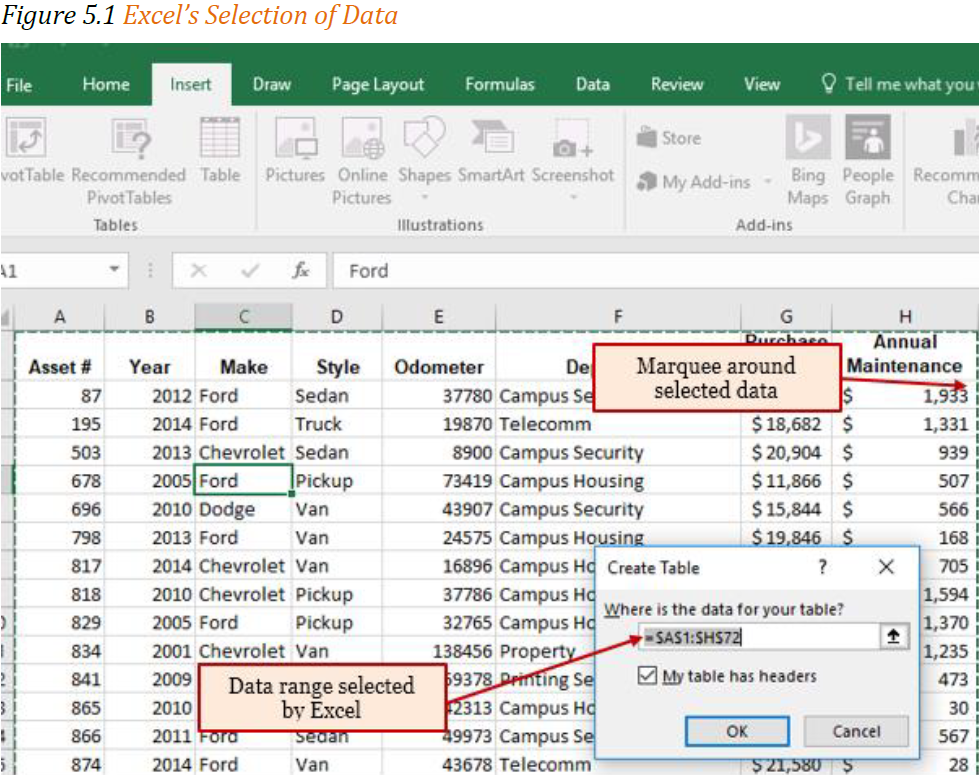
1. From the Create Table dialog box check to make sure it is including all the data table. You will see a marquee around your table and the range selected will be in the dialog box. You can use the dialog box to select the correct data if the range is not correct.

2. Click Ok

Excel will automatically apply a color style with banded rows. We will eliminate the banded rows, because it only adds visual clutter to the data. Remember our data needs to tell a story without clutter. The banded row format will lose the ability to maintain the banded row colors when the table is converted back to a range. Note: we will cover converting back to a range later.

3. In the Table styles section of the Table Tools Design ribbon, use the drop-down in the styles and select None. (Top row, first column) See Figure 5.2. The None style will revert the appearance of your table back to a normal spreadsheet, except that now you will have drop-down arrows next to each of the column headers.

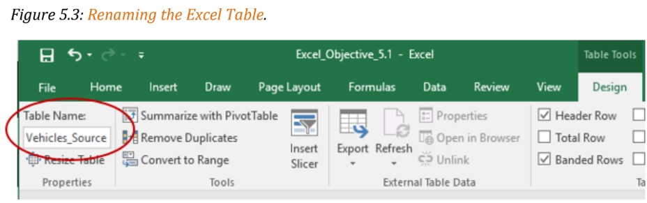
4. Rename the table to Vehicles_Source by clicking in the Table Name Box on the Table Tools ribbon. Note: the same rules that you learned for naming cells and ranges applies to naming tables.

Adding Records

Maintaining data in an Excel table means that you will most likely be adding or deleting records from the table. The simplest way to add a record to an Excel table is to add it at the first blank row at the bottom of the table.

The school recently purchased another vehicle for the maintenance department. The record for the vehicle needs to be added to the Vehicle_Source table. The data for the new vehicle is:

• Asset # 4625

• Year 2023

• Make: Ford

• Style: Pickup

• Odometer: 15

• Department Maintenance

• Purchase price: $44,250

• Annual Maintenance: 2,532

1.From anywhere in the worksheet hold the Ctrl key down and click the End key.

2.Click the Home key to move you to column A.

3.Hit Enter once to move you to the first blank row.

4.Enter the data above. Use the tab key to move you across the cells as you enter the data. Note: as you enter the new data, the table will continue the formatting from the data in the column above the new entry.

Finding and Editing Records

You need to update the records for the 2008 Chevrolet van, asset number 1196, and the 2013 Ford van, asset number 1678. They have been reassigned from Campus Housing to the Athletics department. You’ll use the Find command to locate the records. Then, you will edit the record to change the assigned departments to Athletics.

1. Press the Ctrl+Home keys to move to the top of the worksheet, and then click cell A2 to make it the active cell. You will search on the asset number because it is a distinguishing number in the table.

2. In the Editing group on the Home tab, click the Find & Select button, and then click Find. The Find and Replace dialog box opens.

3. Type 1140 into the Find what: dialog box. Then click Find Next. Leave the Find and Replace dialog box open while you edit the first record.

4. Click F26 and change the department to Athletics. Note: As you type the A, the Athletics department will appear in the auto complete. Hit enter to accept the department.

5. In the Find and Replace dialog box, delete the 1196 asset number and enter the next record number that must be updated, 1678. Click Find Next. Then close the dialog box.

6. Change the department to Athletics.

Deleting Records

The last update required is to delete a record for a sold vehicle. Asset number 1040, a 2003 Ford van was sold and needs to be removed from the asset list.

The steps you will use to delete the record are:

1. Press the Ctrl+Home keys to move to the top of the worksheet, and then click cell A2 to make it the active cell. You will search on the asset number because it is a distinguishing number in the table.

2. In the Editing group on the Home tab, click the Find & Select button, and then click Find. The Find and Replace dialog box opens.

3. Type 1040 into the Find what: dialog box. Then click Find Next. Close the Find and Replace Dialog box.

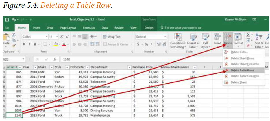
4. In the Cells group of the Home tab, click the Delete button and select Delete Table Rows from the drop down. Note: If a different record was deleted, the active cell was not in the record for the Asset 1140. Click the Undo button and select the correct record.

Adding a Total Row

Follow-along file: Continue with Excel Objective 5.00. (Use file Excel Objective 5.01 if starting here.)

Suni would like to see a count of how many vehicles the college owns. She wants to have the count be dynamically linked to the table contents.

The steps we will use to create a total row, and then change it to a count are:

1. From the Table Style Options on the Table Tools Deign tab, check the box for Total Row. Note: you can uncheck the box to turn off the total row.

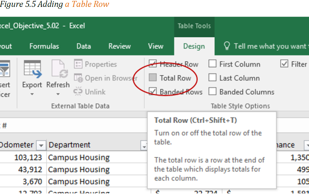
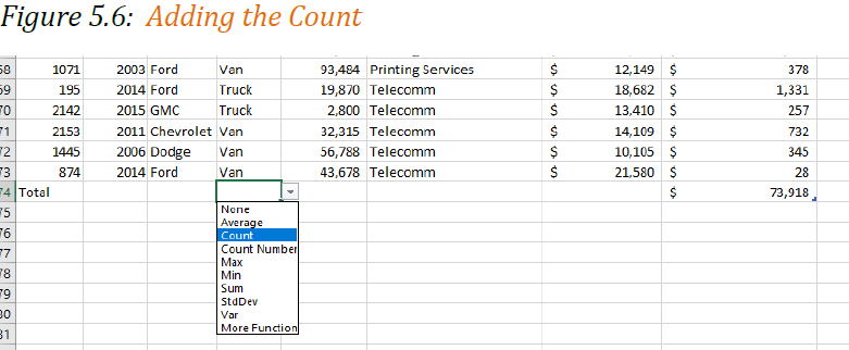
2. Excel will drop you down to the newly created total row. It will automatically put in a total for Annual Maintenance. We will accept that for now. Click on the total row for the Style. From the drop-down select count.

3. Delete the word Total from the A column and type Total number of vehicles. (Don’t worry about overlapping cell walls.)

4. In column g: type Total maintenance.

Remember: Your worksheet must tell a story all by itself!

Adding a New Column

Follow-along file: Continue with Excel Objective 5.00. (Use file Excel Objective 5.02 if starting here.)

Suni would like to see the monthly maintenance cost for each vehicle. She has asked you to add a column next to the Annual Maintenance column.

A unique feature of having your data in a table, versus just a range of data, is the ability to add a column, have the formatting applied, and the formulas added in the top row of the data will automatically copy down the worksheet.

We will add a new column by:

1. Click in cell I1. Type: Monthly Maintenance and hit Enter. The bold and center formatting will automatically be applied to the column header and a drop-down box will appear next to the column header.

2. Resize column I to fit the new header.

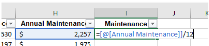
3. In I2 enter a formula to divide the Annual Maintenance by 12. Type = and click on cellH2. Notice that when you click on H2 you see something new in your formula. Instead ofH2 you now see = [@[Annual Maintenance]]. This only occurs in a table. It will allow the formula to be copied down the range of cells in the table automatically. Type /12 after clicking on cell H2.

4. Hit enter to complete the formula.

5. Format the column by clicking on the column header to select it, then click on the lower border of the cell. This will highlight the column data. On the home ribbon select the Accounting format.