12 Lookup Functions
Lookup Functions
Learning Objectives
- Use the VLOOKUP function to search and display the contents of a cell location for data that is organized in columns.
- Use the HLOOKUP function to search and display the contents of a cell location for data that is organized in rows.
- Create a web query that imports stock price data into a worksheet from a website.
The final section of this chapter addresses lookup functions. Lookup functions are typically used to search for and display data located in other worksheets or workbooks. The two lookup functions we will use in our example of the personal investment portfolio are the VLOOKUP and HLOOKUP functions. In addition to demonstrating these functions, we will also show how we can enhance the personal investment portfolio workbook with a web query. Web queries are used to bring live or current data into a worksheet from a website.
The VLOOKUP Function
Follow-along file: Continue with Excel Objective 3.00. (Use file Excel Objective 3.15 if starting here.)
The VLOOKUP function is typically used to access and display data located in another worksheet or workbook. The function can also be used to access and display data located in the same worksheet. This is a very powerful and versatile function because it eliminates the need to copy or recreate data that exists in other worksheets or workbooks.
It is called a VLOOKUP function because the function will search vertically down the first column of a range of cells to find what is called a lookup value. This process is very similar to the statistical IF functions in Section 3.2 “Statistical IF Functions”. You will recall that these functions used criteria to select cells from a range that was used in the mathematical output. The VLOOKUP function is essentially performing the same process; however, instead of selecting multiple cells from a range, the function is only looking for one specific cell location. Once the function finds the specific cell location, it will display the contents of that cell location or another cell location in the range. Before using the VLOOKUP function in the personal investment portfolio workbook, it is strongly recommended that you carefully read the definitions for the function arguments listed in Table 3.10 “Arguments for the VLOOKUP Function”. =VLOOKUP(lookup_value,table_array,row_index_num,[range_lookup])
| Argument | Definition |
| Lookup_value | This argument is typically defined with a cell location, number, or text. Text data must be enclosed in quotation marks for this argument. The function will search for the criteria in the first column of the range used to define the Table_array argument. For example, if the word Hat is used to define this argument, the function will always search for the word Hat in the first column of the range used to define the Table_array argument. |
| Table_array | A range of cells that contain data you wish the VLOOKUP function to search through (Lookup_value) and display. This cell range must contain the criteria used to define the Lookup_value in the first column. |
| Col_index_num | This is the column index number argument. It is defined as the number of columns to the right of the first column in the range used to define the Table_array argument that contains the data you wish to display. For example, suppose the data you wish the function to display is contained in column C. If the range used to define the Table_array argument is A2:D15, then the column index number will be 3. Counting the columns to the right of the first column in this range, Column A would be 1, Column B would be 2, and Column C would be 3. It is important to remember to count the first column in the table array range as 1. |
| [Range_lookup] | This argument is defined with either the word TRUE or the word FALSE. When this argument is defined with the word FALSE, the function will look for an exact match to the criteria used to define the Lookup_value argument in the first column of the table array range. It is important to note the function will search the entire range to find an exact match.
If this argument is defined with the word TRUE, the function will look for a value that is an exact match or the closest match that is less than the lookup value. Examples: If the lookup value is 80 and the highest value in the first column of the table array is a 78, the function will consider 78 a match for the number 80. If the lookup value is 78 and the range is 70, 80, 90, 100, the function will consider 78 to be a match for 70 (the lower value). However, if the lookup value is 80 and the lowest number in the first column of the table array is 85, the function will produce an error. This is because the number 80 and any value less than 80 do not exist in the first column of the table array range. It is important to note that if you define this argument with the word TRUE, the data in the table array must be sorted in ascending order. This is because the function will stop searching for a match once the value in the first column exceeds the lookup value. If the data in the table array is not sorted, the function can either produce an error code or display an erroneous result. This argument is in brackets because if it is not defined it will automatically be defined with the word TRUE. |
Integrity Check – Using a TRUE Range Lookup for VLOOKUP and HLOOKUP
If you are defining the Range_lookup argument with the word TRUE for either the VLOOKUP or HLOOKUP function, the range used to define the Table_array argument must be sorted in ascending order. For the VLOOKUP function, the table array range must be sorted from smallest to largest or from A to Z based on the values in the first column. For the HLOOKUP function, the table array range must be sorted from left to right based on the values in the first row, from smallest to largest or A to Z.
You may have noticed that on the Investment Detail worksheet, the Description column is blank. Descriptions for several investments are included in the workbook in the Investment List worksheet as shown in Figure 3.42 “Investment List Worksheet”. The VLOOKUP function will be used to search for a specific symbol in Column A of the Investment List worksheet and display the description for that symbol located in Column B. It is important to note that once the Table_array has been defined, the VLOOKUP can return any column number within that array. For example, to return the investment type you would select column 3. For 5-year growth, you would select column 6.

Naming a Table_array:
To name a Table_array select all the columns and rows in the array EXCEPT the column headers. If you include the column headers Excel will treat them as values in your array and may return erroneous results.
The following steps explain how to accomplish this:
1. First, we will name our table_array. It is much easier to name the array and use the named range than to constantly have to re-select the data for a different VLOOKUP function.
2. Click on the Investment List worksheet.
3. Select the range A3:F23 (this range excludes the column headers.)
4. On the Formulas ribbon in the Defined Names section click on Define Name.

5. In the Name box type in Investment_List. Notice that the Refers to: box at the bottom shows the worksheet name and range of cells this name will apply to. Make sure it shows the correct range. The $ indicate that naming this range will create an absolute reference to these cells in your workbook.
6. In the Investment Detail worksheet, click on cell C4.
7. Click the Formulas tab on the Ribbon.
8. Click the Lookup & Reference button in the Function Library group of commands.
9. Select the VLOOKUP function from the list of functions. Use the scroll bar to scroll down to the bottom of the list. This will open the Function Arguments dialog box for the VLOOKUP function.
10. Click in the Lookup_value argument on the Function Arguments dialog box.
11. Click cell B4. The symbol in cell B4 is the lookup value that will be searched in the first column of the range defined for the Table_array argument.
12. Click in the Table_array argument on the Function Arguments dialog box.
13. From the Formulas ribbon click on Use in Formula and select Investment_List.
14. Press the TAB key on your keyboard to advance to the Col_index_num argument and type the number 2. Once the function finds the lookup value in the first column of the range Investment_List, it will display the description that is in the second column of the same row.
15. Press the TAB key on your keyboard to advance to the Range_lookup argument and type the word FALSE. This will direct the function to search for only exact matches to lookup value.
16. Click the OK button at the bottom of the Function Arguments dialog box.
17. Copy the VLOOKUP function in cell C4 and paste it into the range C5:C18
Figure 3.43 “Completed Function Arguments Dialog Box for the VLOOKUP Function” shows the completed Function Arguments dialog box for the VLOOKUP function. Notice that the Range_lookup argument is defined with the word FALSE. This will direct the function to search for an exact match to the lookup value and will also direct the function to search the entire first column of the table array range.
Finally, it is important to note the absolute reference on the table array range. This will prevent the table array range from changing when the function is pasted into other cell locations.
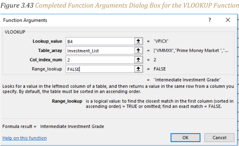
Figure 3.44 “Results of the VLOOKUP Function in the Investment Detail Worksheet” shows the results of the VLOOKUP function in the Investment Detail worksheet. The function is searching for each symbol in Column B of the Investment Detail worksheet in Column A of the Investment List worksheet.
When the function finds a match, it will display whatever is in the cell location two columns to the right, or Column B, in the Investment List worksheet. For example, the symbol VDMIX, which is in cell B8 on the Investment Detail worksheet (see Figure 3.44 “Results of the VLOOKUP Function in the Investment Detail Worksheet”), is also in cell A15 on the Investment List worksheet. As a result, the function is displaying whatever is in cell B15 on the Investment List worksheet, which is the description “Developed Markets.”

Integrity Check – Absolute References on the Table Array Range for the VLOOKUP and HLOOKUP functions
If you have not named your Table_array for the VLOOKUP or HLOOKU functions and will be copying and pasting the VLOOKUP or HLOOKUP function, you will most likely need to place an absolute reference on the range used to define the Table_array argument. If you do not, the table array will change because of relative referencing
The HLOOKUP Function
Follow-along file: Continue with Excel Objective 3.00. (Use file Excel Objective 3.15 if starting here.)
The HLOOKUP function serves the same purpose as the VLOOKUP function. The HLOOKUP function can be used to display data from another worksheet or workbook. However, instead of searching for the lookup value vertically down the first column of the table array range, the HLOOKUP function searches horizontally across the first row of the table array range. When the function finds a match for the lookup value, it will display the contents in a cell location based on a row index number. This number designates which row in the table array range the function should display.
=HLOOKUP(lookup_value,table_array,row_index_num,[range_lookup])
Table 3.11 “Arguments for the HLOOKUP Function” provides a definition for each argument of the HLOOKUP function. It is best to review the definitions of these arguments carefully before using the function.
| Argument | Definition |
| Lookup_value | This argument is typically defined with a cell location, number, or text. Text data must be enclosed in quotation marks for this argument. The function will search for the criteria in the first column of the range used to define the Table_array argument. For example, if the word Hat is used to define this argument, the function will always search for the word Hat in the first column of the range used to define the Table_array argument. |
| Table_array | A range of cells that contain data you wish the HLOOKUP function to search through (Lookup_value) and display. This cell range must contain the criteria used to define the Lookup_value in the first column. For example, if the range A2:D15 is used to define this argument, the criteria used to define the Lookup_value argument must exist in row 2. |
| Row_index_num | This is the row index number argument. It is defined as the number of rows below the the first row in the range used to define the Table_array argument that contains the data you wish to display. For example, suppose the data you wish the function to display is contained in row 5. If the range used to define the Table_array argument is A2:D15, then the row index number will be 4. Counting the rows below the first row in this range, Row 2 would be 1, Row 3 would be 2, Row 4 would be 3, and Row 5 would be 4. It is important to remember to count the first row in the table array range as 1. |
| [Range_lookup] | This argument is defined with either the word TRUE or the word FALSE. When this argument is defined with the word FALSE, the function will look for an exact match to the criteria used to define the Lookup_value argument in the first row of the table array range. It is important to note the function will search the entire range to find an exact match.
If this argument is defined with the word TRUE, the function will look for a value that is an exact match or the closest match that is less than the lookup value. Examples: If the lookup value is 80 and the highest value in the first row of the table array is a 78, the function will consider 78 a match for the number 80. If the lookup value is 78 and the range is 70, 80, 90, 100, the function will consider 78 to be a match for 70 (the lower value). However, if the lookup value is 80 and the lowest number in the first row of the table array is 85, the function will produce an error. This is because the number 80 and any value less than 80 do not exist in the first row of the table array range. It is important to note that if you define this argument with the word TRUE, the data in the table array must be sorted in ascending order from left to right. This is because the function will stop searching for a match once the value in the first row exceeds the lookup value. If the data in the table array is not sorted, the function can either produce an error code or display an erroneous result. This argument is in brackets because if it is not defined it will automatically be defined with the word TRUE. |
The HLOOKUP function will be used on the Portfolio Summary worksheet to display the benchmark growth rates in the range G4:G7. A benchmark is a value that can be used as a standard point of comparison. The Benchmarks worksheet contains growth rates at different year intervals for the benchmarks that will be used to compare the performance for each investment type (see Figure 3.45 “Benchmarks Worksheet”). For the purposes of this workbook, we will be comparing the growth rates for each investment type to the 5- year average growth rate for the benchmarks categories listed in the range H4:H7. The following steps explain how to construct the HLOOKUP function to display the 5-year benchmark values in the Portfolio Summary worksheet:

1. Go to the Benchmarks worksheet by clicking on the Benchmarks tab.
2. We will name the Benchmarks range for use in the HLOOKUP function. The range we will name is B2:E6. The top row contains the look up values the function will use to find a match. The remaining rows will be the results returned once a match is found.
3. Highlight B3:B6 and name the range Benchmarks by typing the name in the Cell address block on the left side of the formula bar.
4. Click cell G4 in the Portfolio Summary worksheet.
5. Click the Formulas tab on the Ribbon.
6. Click the Lookup & Reference button in the Function Library group of commands.
7. Select the HLOOKUP function from the list of functions. This will open the Function Arguments dialog box for the HLOOKUP function.
8. Click in the Lookup_value argument on the Function Arguments dialog box.
9. Click cell H4. The description in cell H4 will be the lookup value that will be searched in the first row of the range defined for the Table_array argument.
10. Click in the Table_array argument on the Function Arguments dialog box.
11. From the Formulas ribbon, Use in Formula, select the named range Benchmarks.
12. Press the TAB key on your keyboard to advance to the Row_index_num argument and type the number 4.

Remember that the Excel row number from the left side of the worksheet window is irrelevant in table arrays. It is the number of rows in the array itself that are counted.
13. Press the TAB key on your keyboard to advance to the Range_lookup argument on the Function Arguments dialog box and type the word FALSE. This will direct the function to search for only exact matches of the lookup value. Without an exact match, the results may be erroneous because Excel will stop looking when it finds an approximate match, or one higher in value.
14. Click the OK button at the bottom of the Function Arguments dialog box.
15. Copy the HLOOKUP function in cell G4 and paste it into the range G5:G7 using the Paste Formulas command.
Figure 3.46 “Completed Function Arguments Dialog Box for the HLOOKUP Function” shows the completed Function Arguments dialog box for the HLOOKUP function. The row index number 4 indicates that the function will display the contents of the cell location in the fourth row of the table array range.

Figure 3.47 “Completed Portfolio Summary Worksheet” shows the output of the HLOOKUP function. Notice that the output of the function in cell G4 is 6.0%. This is because the lookup value was defined with the entry in cell H4, which is the Barclays index. Looking at Figure 3.45 “Benchmarks Worksheet”, if you count the first row of the table array range as Row 1, the value 6.03% is the fourth row in the Barclays column. Since the values in Column G on the Portfolio Summary worksheet are set to 1 decimal place, the value is displayed as 6.0%.

Integrity Check – #N/A and #REF! Errors with Lookup Functions
If you receive the #N/A error code when using the VLOOKUP or HLOOKUP function, it indicates that Excel cannot find the lookup value in the table array range. Check that the lookup value exists in the first column for the VLOOKUP, or the first row for the HLOOKUP, in the range used to define the Table_array argument. You may also see this error code if you copy and paste the function and forget to put an absolute reference on the range used to define the Table_array argument. The #REF! error code indicates that the column index number or row index number exceeds the number of columns or rows in the range used to define the Table_array argument.
IFERROR
Follow-along file: Continue with Excel Objective 3.00. (Use file Excel Objective 3.16 if starting here.)
Suppose your spreadsheet formulas have errors that you anticipate and don’t need to correct, but you want to improve the display of your results. For example, when creating an invoice template you will want the invoice to look blank, but have the functions set up, so that when data is entered into the invoice, the invoice will correctly calculate the amount due. You will want the errors in the functions to not show as errors and not keep Excel from being able to perform the mathematical operations necessary in the invoice.
There are many reasons why formulas can return errors. For example, division by 0 is not allowed, and if you enter the formula =1/0, Excel returns #DIV/0. Error values include #DIV/0!, #N/A, #NAME?, #NULL!, #NUM!, #REF!, and #VALUE!.
| Error Value | Description of Error |
| #DIV/0! | The formula or function contains a number divided by zero. |
| #NAME? | Excel doesn’t recognize text in the formula or function, such as when the function name is misspelled. |
| #NULL! | A formula or function requires two cell ranges to intersect, but they don’t. |
| #NUM! | Invalid numbers are used in a formula or function, such as text entered in a function that requires a number. |
| #REF! | A cell reference used in a formula or function is no longer valid which can occur when a cell used by the function was deleted from the worksheet. |
| #VALUE! | The wrong type of argument is used in a function or formula, which can occur you supply a range of values to a function that requires a single value. |
There are several ways you can hide error messages you are expecting in a worksheet. You can hide error values by converting them to a number such as 0, and then applying a conditional format that hides the value, or by having what looks like a blank cell returned when an error is encountered.
Create an example error
1. Open a blank workbook, or create a new worksheet.
2. Enter 3 in cell B1, enter 0 in cell C1, and in cell A1, enter the formula =B1/C1. The #DIV/0! error appears in cell A1.
3. Select A1, and press F2 to edit the formula.
4. After the equal sign (=), type IFERROR followed by an opening parenthesis. IFERROR(
5. Move the cursor to the end of the formula.
6. Type ,0) – that is, a comma followed by a zero and a closing parenthesis. The formula =B1/C1 becomes =IFERROR(B1/C1,0).
7. Press Enter to complete the formula. The contents of the cell should now display 0 instead of the #DIV! error.
Apply the conditional format
1. Select the cell that contains the error, and on the Home tab, click Conditional Formatting.
2. Click New Rule.
3. In the New Formatting Rule dialog box, click Format only cells that contain.
4. Under Format only cells with, make sure Cell Value appears in the first list box, equal to appears in the second list box, and then type 0 in the text box to the right.
5. Click the Format button.
6. Click the Number tab and then, under Category, click Custom.
7. In the Type box, enter ;;; (three semicolons), and then click OK. Click OK again. The 0 in the cell disappears. This happens because the ;;; custom format causes any numbers in a cell to not be displayed. However, the actual value (0) remains in the cell.
Hide error values by turning the text white
Use the following procedure to format cells that contain errors so that the text in those cells is displayed in a white font. This makes the error text in these cells virtually invisible.
1. Select the range of cells that contain the error value.
2. On the Home tab, in the Styles group, click the arrow next to Conditional Formatting and then click Manage Rules. The Conditional Formatting Rules Manager dialog box appears.
3. Click New Rule. The New Formatting Rule dialog box appears.
4. Under Select a Rule Type, click Format only cells that contain.
5. Under Edit the Rule Description, in the Format only cells with list, select Errors.
6. Click Format, and then click the Font tab.
7. Click the arrow to open the Color list, and under Theme Colors, select the white color.
Hide error values by making the cell look empty
In the error example given above the formula =B1/C1, where the #DIV/0! error appeared in cell A1 we can use quoted in the IFERROR to show a blank cell. The function would then look like =IFERROR(B1/C1,””). The two quotes at the end of the IFERROR will make the cell look blank.
Key Takeaways
- Lookup functions are powerful and versatile tools because they eliminate the need to copy or recreate data that exists in other worksheets or workbooks.
- The VLOOKUP function will look vertically down the first column of the table array range to find the lookup value. The lookup value must exist in the first column of the table array range when using the VLOOKUP function.
- The HLOOKUP function will look horizontally across the first row of the table array range to find the lookup value. The lookup value must exist in the first row of the table array range when using the HLOOKUP function.
- If the Range_lookup argument for the VLOOKUP function is defined with the word TRUE, the data in the table array range must be sorted in ascending order (smallest to largest) based on the values in the first column.
- If the Range_lookup argument for the HLOOKUP function is defined with the word TRUE, the data in the table array range must be sorted in ascending order (smallest to largest), left to right, based on the values in the first row.
- If you are copying and pasting a VLOOKUP or HLOOKUP function to other cell locations in a worksheet, make sure there is a named range or absolute reference placed on the table array range.
- IFERROR can be used in templates to hide the results of formulas that are in cells, but not currently being used.
Sample VLOOKUP Exercise from Microsoft Copilot:
Scenario:
You are given a list of employees with their departments and salaries. You need to find the salary of an employee based on their name and department using the VLOOKUP function combined with the CONCATENATE function.
The CONCATENATE function in Excel is used to join two or more text strings into one string. This function is particularly useful when you need to combine data from different cells into a single cell.
Syntax:
CONCATENATE(text1, [text2], …)
- text1 is the first text string to be joined.
- [text2], … are additional text strings to be joined. You can include up to 255 text arguments.
Step-by-Step Instructions:
- Create the Employee List Table:
-
- In cells A1 to C6, enter the following data:
| A | B | C | |
| 1 | Employee | Department | Salary |
| 2 | John Doe | HR | $50,000 |
| 3 | Jane Smith | IT | $60,000 |
| 4 | Emily Davis | Finance | $55,000 |
| 5 | Michael Brown | IT | $65,000 |
| 6 | Sarah Wilson | HR | $52,000 |
- Create the Lookup Tables:
-
- In cells F1 to H3, enter the following data:
| F | G | H | |
| 1 | Employee | Department | Salary |
| 2 | John Doe | HR | |
| 3 | Michael Brown | IT |
-
- In cells F6 to H8, enter the following data:
| F | G | H | |
| 6 | Employee | Department | Salary |
| 7 | John Doe | HR | |
| 8 | Sarah Wilson | HR |
- Combine Employee and Department Columns:
-
- In cell D2, enter the following formula and drag it down to D6:
- =A2 & ” – ” & B2
- This will create a combined column with the format “Employee – Department”.
- Autofit the column widths as appropriate.
- Sort the table in ascending order by Employee. Your data in A1:D6 should now appear as:
| Employee | Department | Salary | |
| Emily Davis | Finance | $55,000 | Emily Davis – Finance |
| Jane Smith | IT | $60,000 | Jane Smith – IT |
| John Doe | HR | $50,000 | John Doe -HR |
| Michael Brown | IT | $65,000 | Michael Brown -IT |
| Sarah Wilson | HR | $52,000 | Sarah Wilson – HR |
- Add Salary data to column E. Since the lookup value must be in the leftmost column of a table, and column D will be our lookup values, we must copy & paste the Salary data to cells E2:E6.
- Use the VLOOKUP Function without CONCATENATE:
-
- In cell H2, enter the following formula:
- =VLOOKUP(F2, $A$1:$C$6, 2, FALSE)
- Drag the formula down from H2 to H3 to fill in the salaries for the employees.
- Use the VLOOKUP Function with CONCATENATE:
-
- In cell H7, enter the following formula:
- =VLOOKUP(F7 & ” – ” & G7, $D$1:$E$6, 2, FALSE)
- Drag the formula down from H7 to H8 to fill in the salaries for the employees.
Explanation:
- F7 & ” – ” & G7 combines the employee name and department to match the format in the combined column.
- $D$1:$E$6 is the table array (the range of cells that contains the combined data and the salaries).
- 2 is the column index number (the column number in the table array from which to retrieve the value).
- FALSE specifies that you want an exact match.
Expected Result:
After completing the exercise, the salaries for the employees in the lookup table should be filled in as follows:
| F | G | H |
| Employee | Department | Salary |
| John Doe | HR | 50000 |
| Michael Brown | IT | 65000 |
| F | G | H |
| Employee | Department | Salary |
| John Doe | HR | 50000 |
| Sarah Wilson | HR | 52000 |
This exercise demonstrated how to use VLOOKUP with multiple criteria by combining columns.
