4 Printing
Printing
Learning Objectives
1. Use the Page Layout tab to prepare a worksheet forprinting.
2. Add headers and footers to a printed worksheet.
3. Examine how to print worksheets and workbooks.
Once you have completed a workbook, it is good practice to select the appropriate settings for printing. These settings are in the Page Layout tab of the Ribbon and discussed in this section of the chapter.
Page Setup
Follow-along file: Excel Objective 1.0 (Use file Excel Objective 1.14 if starting with this skill.)
Before you can properly print the worksheets in a workbook, you must establish appropriate settings.
The following steps explain several of the commands in the Page Layout tab of the Ribbon used to prepare a worksheet for printing:
- Open the Unit Sales Rank worksheet by left clicking on the worksheet tab.
- Click the Page Layout tab of the Ribbon.
- Click the Margins button in the Page Setup group of commands. This will open a dropdown list of options for setting the margins of your printed document.
- Click the Wide option from the Margins drop-down list.
- Open the Sales by Month worksheet by left clicking on the worksheet tab.
- Click the Page Layout tab of the Ribbon (see Figure 1.62 “Page Layout Commands for Printing”).
- Click the Margins button in the Page Setup group of commands.
- Click the Narrow option from the Margins drop-down list.
- Click the Orientation button in the Page Setup group of commands.
- Click the Landscape option.
- Click the down arrow to the right of the Width button in the Scale to Fit group of commands.
- Click the 1 Page option from the drop-down list.
- Click the down arrow to the right of the Height button in the Scale to Fit group of commands.
- Click the 1 Page option from the drop-down list. This step along with step 12 will automatically reduce the worksheet so that it fits on one piece of paper. It is very common for professionals to create worksheets that fit within the width of the paper being used. However, for long data sets, you may need to set the height to more than one page. Table 1.2 “Printing Resources: Purpose and Use for Page Setup Commands” provides a list of commands found in the Page Layout tab of the Ribbon.
Why Use Print Settings?
Because professionals often share Excel workbooks, it is a good practice to select the
appropriate print settings in the Page Layout tab even if you do not intend to print the
worksheets in a workbook. It can be extremely frustrating for recipients of a workbook
who wish to print your worksheets to find that the necessary print settings have not
been selected. This may reflect poorly on your attention to detail, especially if the
recipient of the workbook is your boss.
| Command | Purpose | Use |
| Margins | Sets the top, bottom, right, and left margin space for the printed document. | 1. Click the Page Layout tab.
2. Click the Margin button. 3. Click one of the preset margin |
| Orientation | Sets the orientation of the printed document to either portrait or landscape. | 1. Click the Page Layout tab of the Ribbon.
2. Click the Orientation button. 3. Click one of the preset orientation |
| Size | Sets the paper size for the printed document. | 1. Click the Page Layout tab of the Ribbon.
2. Click the Size button. 3. Click one of the preset paper size |
| Print Area | Used for printing only a specific area or range of cells on a worksheet. | 1. Highlight the range of cells on a worksheet that you wish to print.
2. Click the Page Layout tab of the Ribbon. 3. Click the Print Area button. 4. Click the Set Print Area option from the drop-down list. |
| Breaks | Allows you to manually set the page breaks on a worksheet. | 1. Activate a cell on the worksheet where the page break should be placed. Breaks are created above and to the left of the activated cell.
2. Click the Page Layout tab of the Ribbon. 3. Click the Breaks button. 4. Click the Insert Page Break option |
| Background | Adds a picture behind the cell locations in a worksheet. | 1. Click the Page Layout tab of the Ribbon.
2. Click the Background button. 3. Select a picture stored on your computer or network. |
| Print Titles | Used when printing large data sets that are several pages long. This command will repeat the column headings at the top of each printed page. | 1. Click the Page Layout tab of the Ribbon.
2. Click the Print Titles button. 3. Click in the Rows to Repeat at Top input box in the Page Setup dialog box. 4. Click any cell in the row that contains the column headings for your worksheet. 5. Click the OK button at the bottom of |
Headers and Footers
Follow-along file: Excel Objective 1.0 (Use file Excel Objective 1.15 if you are starting with this skill.)
When printing worksheets from Excel, it is common to add headers and footers to the printed document. Information in the header or footer could include the date, page number, file name, company name, and so on. The following steps explain how to add headers and footers to the Excel Objective 1.0 workbook:
- Open the Unit Sales Rank worksheet by left clicking on the worksheet tab.
- Click the Insert tab of the Ribbon. (Make sure your Excel window is maximized)
- Click the Header & Footer button in the Text group of commands. You will see the Design tab added to the Ribbon; this is used for creating the headers and footers for the printed worksheet. Also, this will convert the view of the worksheet from Normal to Page Layout (see Figure 1.63 “Design Tab for Creating Headers and Footers”).
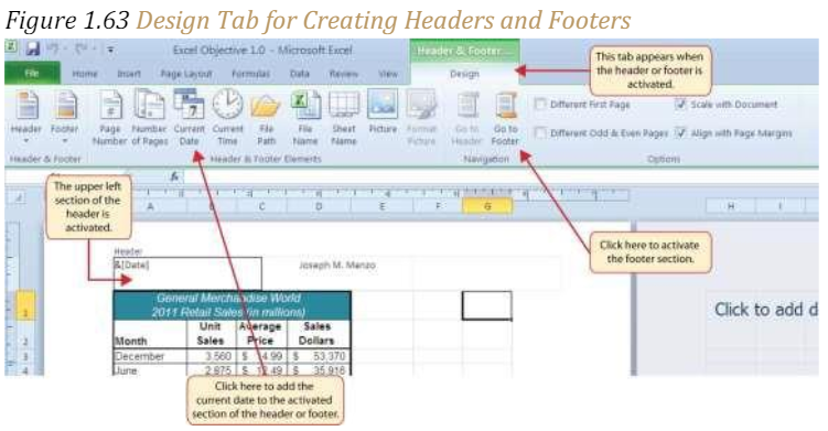
- Type your name in the center section of the Header.
- Place the mouse pointer over the left section of the Header and left click (see Figure 1.63 “Design Tab for Creating Headers and Footers”).
- Click the Current Date button in the Header & Footer Elements group of commands in the Design tab of the Ribbon.
- Click the Go to Footer button in the Navigation group of commands in the Design tab of the Ribbon.
- Place the mouse pointer over the far-right section of the footer and left click.
- Click the Page Number button in the Header & Footer Elements group of commands in the Design tab of the Ribbon.
- Click any cell location outside the header or footer area. The Design tab for creating headers and footers will disappear.
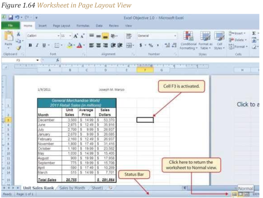
- Click the Normal view button in the lower right side of the Status Bar (see Figure 1.64 “Worksheet in Page Layout View”).
- Open the Sales by Month worksheet by left clicking the worksheet tab.
- Repeat steps 2 through 11 to create the same header and footer for this worksheet.
Printing Worksheets and Workbooks
Follow-along file: Excel Objective 1.0 (Use file Excel Objective 1.16 if starting with this skill.)
Once you have established the print settings for the worksheets in a workbook and have added headers and footers, you are ready to print your worksheets. The following steps explain how to print the worksheets in the Excel Objective 1.0 workbook:
1. Open the Unit Sales Rank worksheet by left clicking on the worksheet tab.
2. Click the File tab on the Ribbon.
3. Click the Print option on the left side of the Backstage view (see Figure 1.65 “Print Preview”). On the right side of the Backstage view, you will be able to see a preview of your printed worksheet.
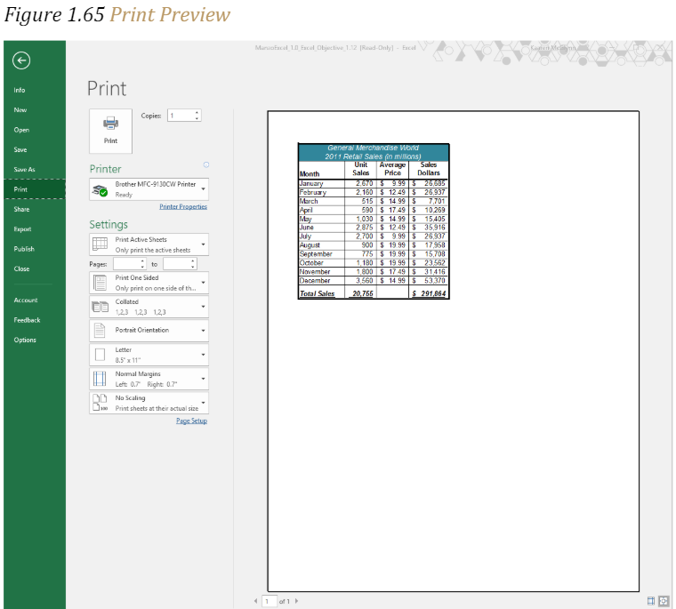
4. Click the Print Active Sheets button in the Print section of the Backstage view (see Figure 1.65 “Print Preview”).
5. Click the Print Entire Workbook option from the drop-down list. This will print all worksheets in a workbook when the Print button is clicked.
6. Click the Next Page arrow at the bottom of the preview window.
7. Click the Print button.
8. Click the Home tab of the Ribbon.
9. Save and close the Excel Objective 1.0 workbook.
Key Takeaways
• The commands in the Page Layout tab of the Ribbon are used to prepare a worksheet
for printing.
• You can add headers and footers to a worksheet to show key information such as
page numbers, the date, the file name, your name, and so on.
• The Print commands are in the File tab of the Ribbon.
Chap 1 Sample Exercise
Creating and maintaining budgets are common practices in many careers. Budgets play a critical role in helping a business or household control expenditures. In this exercise, you will create a budget for a hypothetical medical office.
Begin the exercise by opening the file named Chapter 1 CiP Exercise 1.
- Activate all the cell locations in the Sheet1 worksheet by left clicking the Select All button in the upper left corner of the worksheet.
- In the Home tab of the Ribbon, set the font style to Arial and the font size to 12 points.
- Increase the width of Column A so all the entries in the range A3:A8 are visible. Place the mouse pointer between the letter A and letter B of Column A and Column B. When the mouse pointer changes to a double arrow, left click and drag it to the right until the character width is 18.00.
- Enter Quarter 1 in cell B2.
- Use Auto fill to complete the headings in the range C2:E2. Activate cell B2 and place the mouse pointer over the Fill Handle. When the mouse pointer changes to a black plus sign, left click and drag it to cell E2.
- Increase the width of Columns B, C, D, and E to 10.14 characters. Highlight the range B2:E2 and click the Format button in the Home tab of the Ribbon. Click the Column Width option, type 10.14 in the Column Width dialog box, and then click the OK button in the Column Width dialog box.
- Make the following format adjustment to the range A2:E2: bold; and change the cell fill color to orange.
- Set the alignment in cell B2 to Wrap Text. Activate the cell location and click the Wrap Text button in the Home tab of the Ribbon.
- Copy cell B3 and paste the contents into the range C3:E3.
- Copy the contents in the range B6:B8 by highlighting the range and clicking the Copy button in the Home tab of the Ribbon. Then, highlight the range C6:E8 and click the Paste button in the Home tab of the Ribbon.
- Insert a blank column between Columns A and B. Activate any cell location in Column B. Then, click the drop-down arrow of the Insert button in the Home tab of the Ribbon. Click the Insert Sheet Columns option. (Alternatively, you can right click and insert column.)
- Adjust the width of Column B to 13.29 characters.
- Enter the words Budget Cost in cell B2.
- Calculate the total budget for all four quarters for the salaries. Activate cell B3 and click the down arrow on the AutoSum button in the Formulas tab of the Ribbon. Click the Sum option from the drop- down list. Then, highlight the range C3:F3 and press the ENTER key on your keyboard.
- Copy the contents of cell B3 and paste them into the range B4:B8.
- Enter the words Medical Office Budget in cell A1.
- Merge the cells in the range A1:F1. Highlight the range and click the Merge & Center button in the Home tab of the Ribbon.
- Make the following format adjustments to the range A1:F1: bold; italics; change the font size to 14 points; change the cell fill color to Blue, Accent 1, Darker 50%; and change the font color to white.
- Increase the height of Row 1 to fit the title.
- Sort the data in the range A2:F8 based on the values in the Quarter 4 column in ascending order. Have an active cell anywhere in the range A2:F8 and click the Sort button in the Data tab of the Ribbon. Select Quarter 4 in the “Sort by” drop-down box and select Smallest to Largest in the Order drop-down box. Click the OK button. (Because you have inserted a merged cell title you will need to select the data you want to sort.)
- Format the range B3:F8 with a US dollar sign and zero decimal places.
- Add vertical and horizontal lines to the range A1:F8. Highlight the range and click the down arrow next to the Borders button in the Home tab of the Ribbon.
- Select the All Borders option from the drop-down list.
- Change the name of the Sheet1 worksheet tab to “Budget.” Double click the worksheet tab, type the word Budget, and press the ENTER key.
- Insert a pie chart using the data in the range A2:B8. Highlight the range and click the Pie button in the Insert tab of the Ribbon. Click the first option on the list (the Pie option).
- Click and drag the chart so the upper left corner is in the center of cell H2.
- Add labels to the chart by clicking the Layout 1 option from the Chart Layouts list in the Design tab of the Ribbon. Make sure the chart is activated by clicking it once before you look for the Layout 1 Chart Layout option.
- Change the orientation of the Budget worksheet so it prints landscape instead of portrait.
- Adjust the appropriate settings so the Budget worksheet prints on one piece of paper.
- Add a header to the Budget worksheet that shows the date in the upper left corner and your name in the center.
- Add a footer to the Budget worksheet that shows the page number in the lower right corner.
- Use the Save As command in the File tab of the Ribbon to save the workbook by adding your name in front of the current workbook name (i.e., “your name Chapter 1 CiP Exercise 1”).
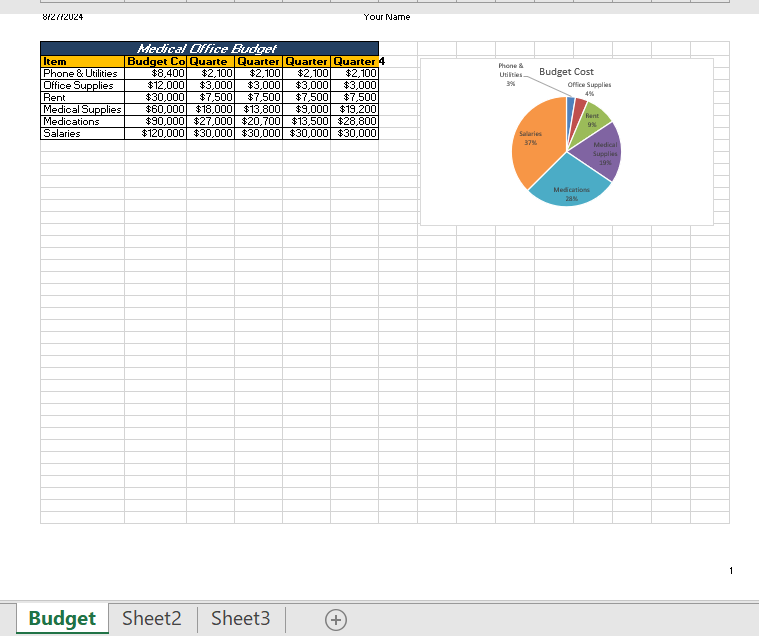
- Close the workbook and Excel. Compare your results with the figure below.
Figure 1 – Completed Medical Budget Exercise
Media Attributions
- Excel Help
